Stochastic Differential Equations: From Mathematical Foundations to Modern Applications
An intuitive tour of Brownian motion, Ito calculus, and how stochastic differential equations model systems that evolve randomly over time.
Mathematics
Finance
Machine Learning
Python
Stochastic Processes
Author
Jan Schlegel
Published
April 3, 2025
Abstract
This comprehensive treatment of stochastic differential equation theory covers fundamental concepts from Brownian motion and Itô calculus to advanced applications in mathematical finance, neural processes, and diffusion models. We provide rigorous mathematical foundations, numerical solution methods, and extensive Python implementations with publication-ready visualizations, bridging classical stochastic analysis with cutting-edge machine learning applications.
Stochastic differential equations provide the mathematical framework for modeling continuous-time random processes, with applications spanning from option pricing to generative AI models
1 Introduction
Stochastic differential equations (SDEs) represent one of the most profound and mathematically elegant frameworks in modern probability theory and applied mathematics. These equations describe the evolution of random processes in continuous time, providing the mathematical foundation for modeling phenomena characterized by both deterministic trends and random fluctuations [@oksendal2003; @karatzas1991].
The theoretical development of SDE theory emerged from the intersection of probability theory, differential equations, and mathematical finance, culminating in the revolutionary work of Kiyoshi Itô in the 1940s. Itô’s groundbreaking construction of stochastic integration transformed our understanding of random processes and established the mathematical framework that now underpins modern quantitative finance, statistical physics, and machine learning [@ito1951; @mckean1969].
1.1 Historical Development and Motivation
The genesis of stochastic differential equations can be traced to Louis Bachelier’s pioneering 1900 thesis on option pricing, where he first applied Brownian motion to financial markets [@bachelier1900]. However, it was not until Norbert Wiener’s rigorous mathematical construction of Brownian motion in the 1920s that the field gained its theoretical foundation [@wiener1923].
The transformative breakthrough came with Itô’s development of stochastic calculus in the 1940s and 1950s. Itô recognized that classical calculus was inadequate for handling functions of Brownian motion due to their non-differentiable nature, leading to his construction of stochastic integration and the famous Itô’s lemma [@ito1951]. This work established the mathematical machinery necessary for:
Rigorous treatment of random processes: Moving beyond heuristic arguments to mathematically precise formulations
Financial modeling: Providing the foundation for modern option pricing theory through the Black-Scholes model
Engineering applications: Enabling analysis of systems subject to random disturbances
Machine learning: Supporting modern developments in neural differential equations and diffusion models
1.2 Contemporary Relevance and Applications
In the 21st century, SDEs have experienced a renaissance driven by advances in computational methods and emerging applications in machine learning. Key contemporary developments include:
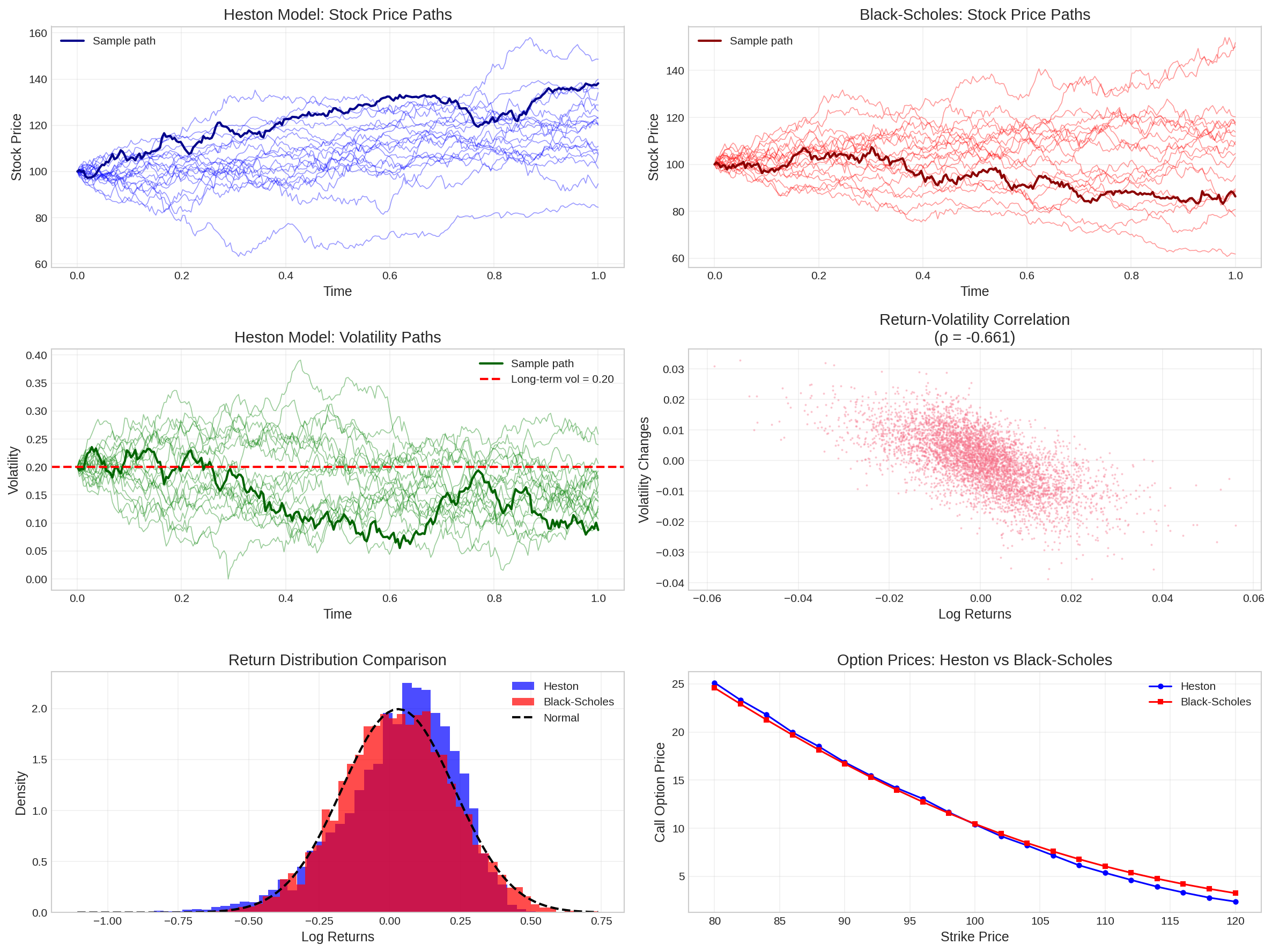
Mathematical Finance: SDEs form the backbone of modern derivatives pricing, risk management, and portfolio optimization. Models like the Heston stochastic volatility model and interest rate models (Vasicek, Cox-Ingersoll-Ross) are built on SDE foundations [@heston1993; @cox1985].
Machine Learning and AI: Recent breakthroughs in generative modeling, particularly diffusion models for image generation, rely heavily on SDE theory. Neural ordinary differential equations (NODEs) and neural SDEs represent cutting-edge applications of stochastic analysis to deep learning [@chen2018; @song2021].
Scientific Computing: SDEs provide essential tools for modeling complex systems in physics, biology, and engineering where random effects play a crucial role [@gardiner2009].
1.3 Scope and Mathematical Prerequisites
This treatise provides a comprehensive, PhD-level treatment of stochastic differential equation theory and applications. We assume familiarity with:
Real analysis: Measure theory, Lebesgue integration, and functional analysis
Probability theory: Probability spaces, random variables, and basic stochastic processes
Differential equations: Ordinary differential equations and partial differential equations
Linear algebra: Matrix theory and spectral analysis
Our systematic development progresses through:
Theoretical Foundations (Sections 2-4): We establish the mathematical framework, beginning with Brownian motion and filtrations, developing Itô calculus, and proving fundamental existence and uniqueness theorems.
Numerical Methods (Section 5): We examine computational approaches including Euler-Maruyama and Milstein schemes, analyzing convergence properties and implementation considerations.
Financial Applications (Section 6): We explore classical applications in option pricing, interest rate modeling, and risk management, providing complete derivations and implementations.
Modern Machine Learning Applications (Sections 7-8): We investigate contemporary applications in neural differential equations, diffusion models, and Gaussian processes, connecting classical theory to cutting-edge developments.
Advanced Topics (Section 9): We cover jump-diffusion processes, stochastic volatility models, and path-dependent derivatives.
Throughout, we provide rigorous mathematical proofs, comprehensive Python implementations optimized with modern computational libraries, and publication-quality visualizations that illuminate key concepts and facilitate practical application.
2 Mathematical Foundations
2.1 Probability Spaces and Filtrations
The rigorous development of stochastic differential equation theory requires careful construction of the underlying probability framework. We begin with the fundamental mathematical structures that support stochastic analysis.
Definition 2.1 (Probability Space): A probability space is a triple \((\Omega, \mathcal{F}, \mathbb{P})\) where: - \(\Omega\) is the sample space representing all possible outcomes - \(\mathcal{F}\) is a \(\sigma\)-algebra on \(\Omega\) representing measurable events - \(\mathbb{P}: \mathcal{F} \to [0,1]\) is a probability measure satisfying \(\mathbb{P}(\Omega) = 1\)
Definition 2.2 (Filtration): A filtration \(\{\mathcal{F}_t\}_{t \geq 0}\) is an increasing family of sub-\(\sigma\)-algebras of \(\mathcal{F}\): \[\mathcal{F}_s \subseteq \mathcal{F}_t \subseteq \mathcal{F} \quad \text{for all } 0 \leq s \leq t\]
The filtration represents the evolution of information over time, where \(\mathcal{F}_t\) contains all events observable up to time \(t\).
2.2 Brownian Motion and the Wiener Process
Brownian motion forms the cornerstone of stochastic calculus, providing the fundamental building block for constructing more complex stochastic processes.
Definition 2.3 (Standard Brownian Motion): A stochastic process \(\{W_t\}_{t \geq 0}\) defined on \((\Omega, \mathcal{F}, \mathbb{P})\) is called standard Brownian motion if:
Initial condition: \(W_0 = 0\) almost surely
Independent increments: For any \(0 \leq t_1 < t_2 < \cdots < t_n\), the increments \(W_{t_2} - W_{t_1}, W_{t_3} - W_{t_2}, \ldots, W_{t_n} - W_{t_{n-1}}\) are independent
Gaussian increments: For any \(s < t\), \(W_t - W_s \sim \mathcal{N}(0, t-s)\)
Continuous paths: \(t \mapsto W_t(\omega)\) is continuous for almost all \(\omega \in \Omega\)
Code
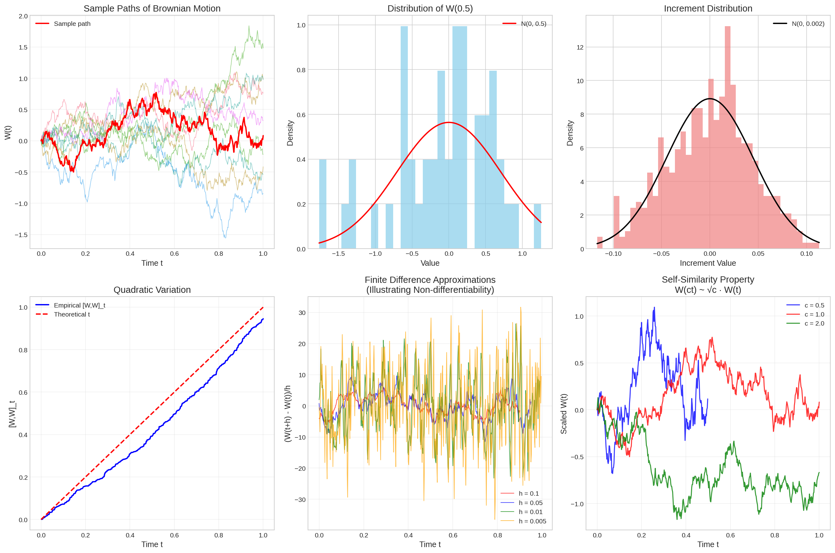
@njitdef simulate_brownian_motion(T, N, n_paths=5):"""Efficiently simulate Brownian motion paths using Numba acceleration.""" dt = T / N sqrt_dt = np.sqrt(dt) paths = np.zeros((n_paths, N +1))for i inrange(n_paths):for j inrange(1, N +1): paths[i, j] = paths[i, j-1] + sqrt_dt * np.random.randn()return paths# Simulation parametersT =1.0# Time horizonN =500# Number of time steps (reduced for faster rendering)n_paths =50# Reduced number of pathsdt = T / Nt = np.linspace(0, T, N +1)# Generate multiple Brownian motion pathsnp.random.seed(42)paths = simulate_brownian_motion(T, N, n_paths)fig, axes = plt.subplots(2, 3, figsize=(18, 12))# Sample pathsaxes[0, 0].plot(t, paths[:10].T, alpha=0.6, linewidth=0.8)axes[0, 0].plot(t, paths[0], 'r-', linewidth=2, label='Sample path')axes[0, 0].set_title('Sample Paths of Brownian Motion')axes[0, 0].set_xlabel('Time t')axes[0, 0].set_ylabel('W(t)')axes[0, 0].legend()axes[0, 0].grid(True, alpha=0.3)# Distribution at fixed timet_fixed =0.5W_fixed = paths[:, int(t_fixed * N)]axes[0, 1].hist(W_fixed, bins=30, density=True, alpha=0.7, color='skyblue')x_range = np.linspace(W_fixed.min(), W_fixed.max(), 100)theoretical_pdf = stats.norm.pdf(x_range, 0, np.sqrt(t_fixed))axes[0, 1].plot(x_range, theoretical_pdf, 'r-', linewidth=2, label=f'N(0, {t_fixed})')axes[0, 1].set_title(f'Distribution of W({t_fixed})')axes[0, 1].set_xlabel('Value')axes[0, 1].set_ylabel('Density')axes[0, 1].legend()# Increment distributionincrements = np.diff(paths[0])axes[0, 2].hist(increments, bins=40, density=True, alpha=0.7, color='lightcoral')x_inc = np.linspace(increments.min(), increments.max(), 100)theoretical_inc = stats.norm.pdf(x_inc, 0, np.sqrt(dt))axes[0, 2].plot(x_inc, theoretical_inc, 'k-', linewidth=2, label=f'N(0, {dt:.3f})')axes[0, 2].set_title('Increment Distribution')axes[0, 2].set_xlabel('Increment Value')axes[0, 2].set_ylabel('Density')axes[0, 2].legend()# Quadratic variation approximationdef quadratic_variation(path, dt):"""Compute empirical quadratic variation.""" increments = np.diff(path)return np.cumsum(increments**2)qv = quadratic_variation(paths[0], dt)axes[1, 0].plot(t[1:], qv, 'b-', linewidth=2, label='Empirical [W,W]_t')axes[1, 0].plot(t, t, 'r--', linewidth=2, label='Theoretical t')axes[1, 0].set_title('Quadratic Variation')axes[1, 0].set_xlabel('Time t')axes[1, 0].set_ylabel('[W,W]_t')axes[1, 0].legend()axes[1, 0].grid(True, alpha=0.3)# Path roughness (non-differentiability)# Compute finite difference approximations to derivativesh_values = [0.1, 0.05, 0.01, 0.005]colors = ['red', 'blue', 'green', 'orange']for i, h inenumerate(h_values): n_h =int(h / dt)if n_h >0: t_deriv = t[:-n_h] finite_diff = (paths[0, n_h:] - paths[0, :-n_h]) / h axes[1, 1].plot(t_deriv, finite_diff, color=colors[i], alpha=0.7, linewidth=1, label=f'h = {h}')axes[1, 1].set_title('Finite Difference Approximations\n(Illustrating Non-differentiability)')axes[1, 1].set_xlabel('Time t')axes[1, 1].set_ylabel('(W(t+h) - W(t))/h')axes[1, 1].legend()axes[1, 1].grid(True, alpha=0.3)# Scaling property demonstrationscaled_paths = []scale_factors = [0.5, 1.0, 2.0]colors_scale = ['blue', 'red', 'green']for i, c inenumerate(scale_factors):# W(ct) has same distribution as sqrt(c) * W(t)if c !=1.0: t_scaled = t * cif c <1.0:# Subsample for c < 1 indices = np.linspace(0, len(t)-1, int(len(t)*c)).astype(int) scaled_path = paths[0, indices] / np.sqrt(c) t_plot = t[:len(indices)]else:# Extend time for c > 1 (simplified for faster rendering) extended_path = simulate_brownian_motion(T*c, int(N*c*0.5), 1)[0] scaled_path = extended_path / np.sqrt(c) t_plot = np.linspace(0, T, len(scaled_path))else: scaled_path = paths[0] t_plot = t axes[1, 2].plot(t_plot, scaled_path, color=colors_scale[i], linewidth=1.5, alpha=0.8, label=f'c = {c}')axes[1, 2].set_title('Self-Similarity Property\nW(ct) ~ √c · W(t)')axes[1, 2].set_xlabel('Time t')axes[1, 2].set_ylabel('Scaled W(t)')axes[1, 2].legend()axes[1, 2].grid(True, alpha=0.3)plt.tight_layout()plt.show()
Figure 1: Sample paths of Brownian motion and their key properties
Theorem 2.4 (Properties of Brownian Motion): Standard Brownian motion possesses the following fundamental properties:
Martingale property: \(\{W_t\}\) is a martingale with respect to its natural filtration
Quadratic variation: \([W,W]_t = t\) (in the sense of convergence in probability)
Self-similarity: \(\{W_{ct}\}_{t \geq 0} \stackrel{d}{=} \{\sqrt{c} W_t\}_{t \geq 0}\) for any \(c > 0\)
Path properties: Paths are continuous but nowhere differentiable with probability 1
2.3 Multi-dimensional Brownian Motion
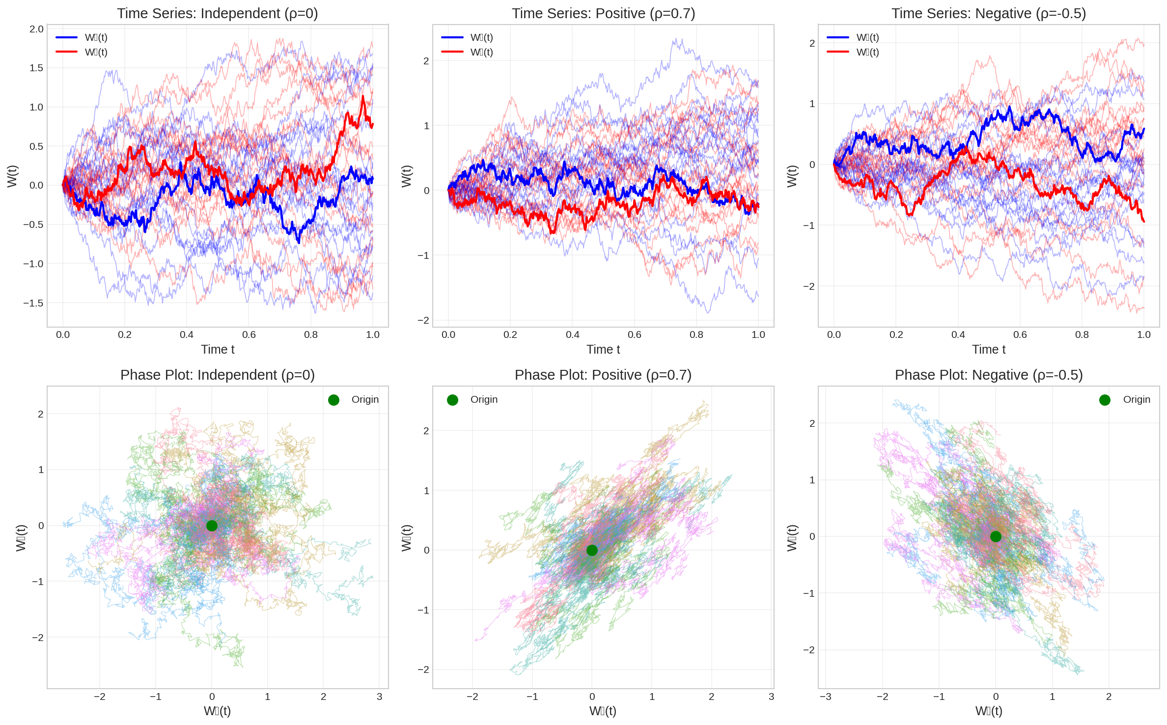
Definition 2.5 (d-dimensional Brownian Motion): A \(d\)-dimensional Brownian motion is a vector process \(\mathbf{W}_t = (W_t^{(1)}, \ldots, W_t^{(d)})^T\) where each component \(W_t^{(i)}\) is independent standard Brownian motion.
For correlated Brownian motions, we can construct them using: \[\mathbf{W}_t = \mathbf{L} \mathbf{Z}_t\] where \(\mathbf{Z}_t\) is \(d\)-dimensional independent Brownian motion and \(\mathbf{L}\) is the Cholesky decomposition of the correlation matrix \(\boldsymbol{\Sigma}\).
Figure 2: Multi-dimensional Brownian motion with correlation structure
2.4 Martingales and Stopping Times
Definition 2.6 (Martingale): A stochastic process \(\{M_t\}_{t \geq 0}\) adapted to filtration \(\{\mathcal{F}_t\}\) is a martingale if: 1. \(\mathbb{E}[|M_t|] < \infty\) for all \(t \geq 0\) 2. \(\mathbb{E}[M_t | \mathcal{F}_s] = M_s\) for all \(0 \leq s \leq t\)
Theorem 2.7 (Examples of Martingales): The following processes are martingales: 1. Brownian motion \(W_t\) 2. \(W_t^2 - t\) (compensated quadratic variation) 3. \(\exp(\sigma W_t - \frac{\sigma^2 t}{2})\) for any \(\sigma \in \mathbb{R}\) (exponential martingale)
Definition 2.8 (Stopping Time): A random variable \(\tau: \Omega \to [0, \infty]\) is a stopping time with respect to \(\{\mathcal{F}_t\}\) if for every \(t \geq 0\): \[\{\tau \leq t\} \in \mathcal{F}_t\]
Theorem 2.9 (Optional Stopping Theorem): If \(M_t\) is a martingale and \(\tau\) is a bounded stopping time, then: \[\mathbb{E}[M_\tau] = \mathbb{E}[M_0]\]
These foundational concepts provide the mathematical infrastructure necessary for constructing stochastic integrals and developing the theory of stochastic differential equations. In the next section, we will build upon this foundation to develop Itô calculus, the cornerstone of stochastic analysis.
3 Itô Calculus and Stochastic Integration
The development of stochastic calculus represents one of the most profound mathematical achievements of the 20th century. Classical calculus fails when applied to functions of Brownian motion due to their infinite variation and non-differentiable nature. Itô’s revolutionary insight was to develop a new form of calculus specifically designed for stochastic processes.
3.1 The Need for Stochastic Calculus
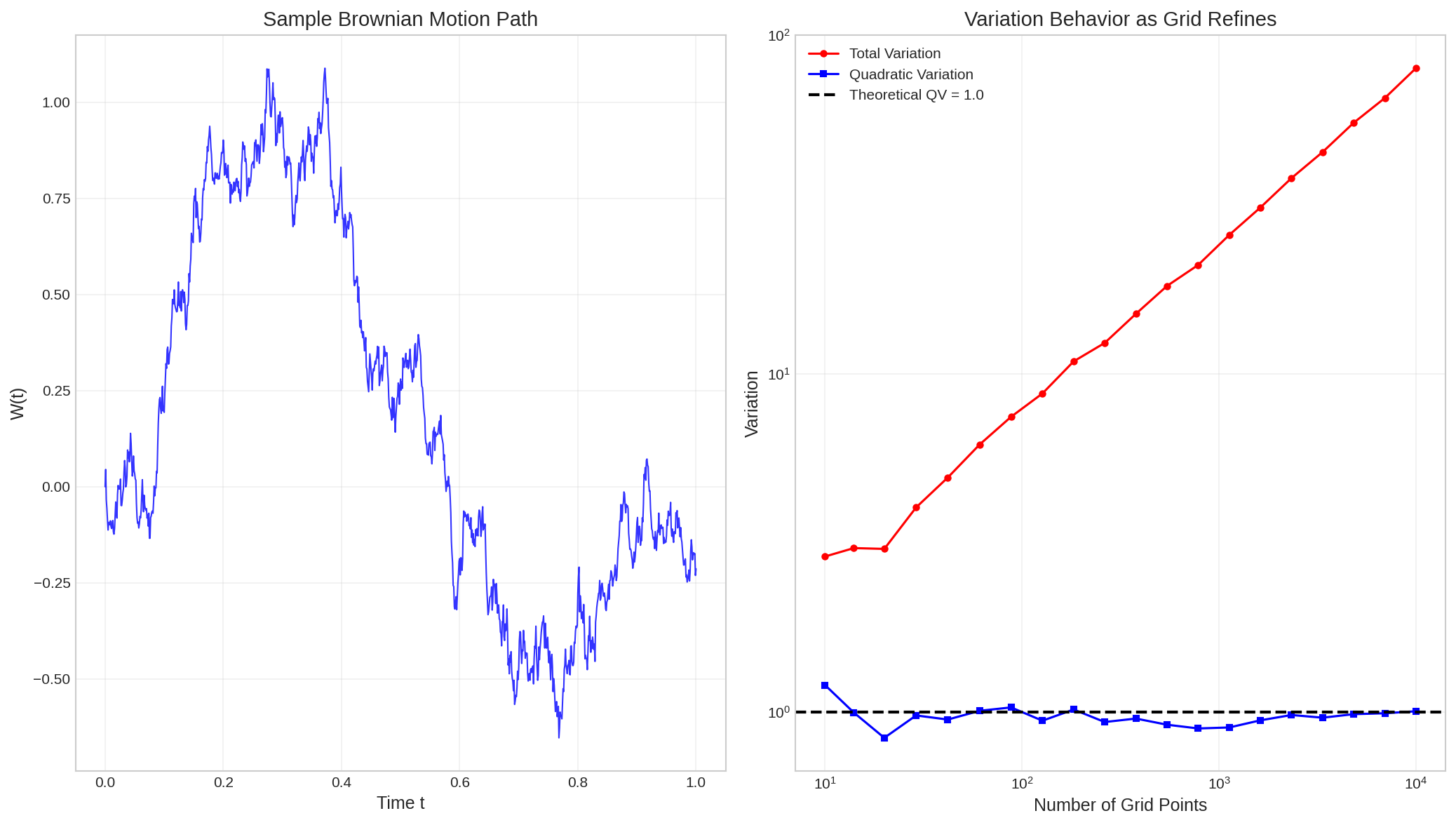
Consider attempting to define the integral \(\int_0^t W_s \, dW_s\) using classical Riemann-Stieltjes integration. The fundamental problem arises from the fact that Brownian motion has infinite variation on any interval, making classical integration impossible.
Code
def compute_variation(path, time_grid):"""Compute total variation of a function on given grid."""return np.sum(np.abs(np.diff(path)))def compute_quadratic_variation(path, time_grid):"""Compute quadratic variation approximation."""return np.sum(np.diff(path)**2)# Generate fine Brownian motion pathT =1.0N_fine =10000t_fine = np.linspace(0, T, N_fine +1)dt_fine = T / N_finenp.random.seed(42)W_fine = np.cumsum(np.concatenate([[0], np.random.randn(N_fine) * np.sqrt(dt_fine)]))# Compute variations for different grid sizesgrid_sizes = np.logspace(1, 4, 20).astype(int)total_variations = []quadratic_variations = []for N in grid_sizes:if N <= N_fine: indices = np.linspace(0, N_fine, N +1).astype(int) subpath = W_fine[indices] t_sub = t_fine[indices] total_var = compute_variation(subpath, t_sub) quad_var = compute_quadratic_variation(subpath, t_sub) total_variations.append(total_var) quadratic_variations.append(quad_var)fig, axes = plt.subplots(1, 2, figsize=(14, 8))# Plot path and variationsN_display =1000indices = np.linspace(0, N_fine, N_display +1).astype(int)axes[0].plot(t_fine[indices], W_fine[indices], 'b-', linewidth=1, alpha=0.8)axes[0].set_title('Sample Brownian Motion Path')axes[0].set_xlabel('Time t')axes[0].set_ylabel('W(t)')axes[0].grid(True, alpha=0.3)# Plot variation convergenceaxes[1].loglog(grid_sizes[:len(total_variations)], total_variations, 'ro-', label='Total Variation', markersize=4)axes[1].loglog(grid_sizes[:len(quadratic_variations)], quadratic_variations, 'bs-', label='Quadratic Variation', markersize=4)axes[1].axhline(y=T, color='black', linestyle='--', linewidth=2, label=f'Theoretical QV = {T}')axes[1].set_xlabel('Number of Grid Points')axes[1].set_ylabel('Variation')axes[1].set_title('Variation Behavior as Grid Refines')axes[1].legend()axes[1].grid(True, alpha=0.3)plt.tight_layout()plt.show()print(f"Final total variation: {total_variations[-1]:.2f}")print(f"Final quadratic variation: {quadratic_variations[-1]:.3f}")print(f"Theoretical quadratic variation: {T}")
Figure 3: Illustration of infinite variation in Brownian motion
Final total variation: 79.95
Final quadratic variation: 1.007
Theoretical quadratic variation: 1.0
3.2 Construction of the Itô Integral
Definition 3.1 (Simple Process): A stochastic process \(\{H_t\}\) is simple if it can be written as: \[H_t = H_0 \mathbf{1}_{\{0\}}(t) + \sum_{i=1}^n H_{t_i} \mathbf{1}_{(t_i, t_{i+1}]}(t)\] where \(0 = t_0 < t_1 < \cdots < t_n < \infty\) and each \(H_{t_i}\) is \(\mathcal{F}_{t_i}\)-measurable.
Definition 3.2 (Itô Integral for Simple Processes): For a simple process \(H_t\), the Itô integral is defined as: \[\int_0^t H_s \, dW_s = \sum_{i=0}^{n-1} H_{t_i}(W_{t_{i+1} \wedge t} - W_{t_i \wedge t})\]
Definition 3.4 (General Itô Integral): For adapted processes \(H_t\) satisfying \(\mathbb{E}\left[\int_0^t H_s^2 \, ds\right] < \infty\), the Itô integral \(\int_0^t H_s \, dW_s\) is defined as the \(L^2\) limit of Itô integrals of simple processes approximating \(H_t\).
3.3 Itô’s Lemma: The Fundamental Theorem
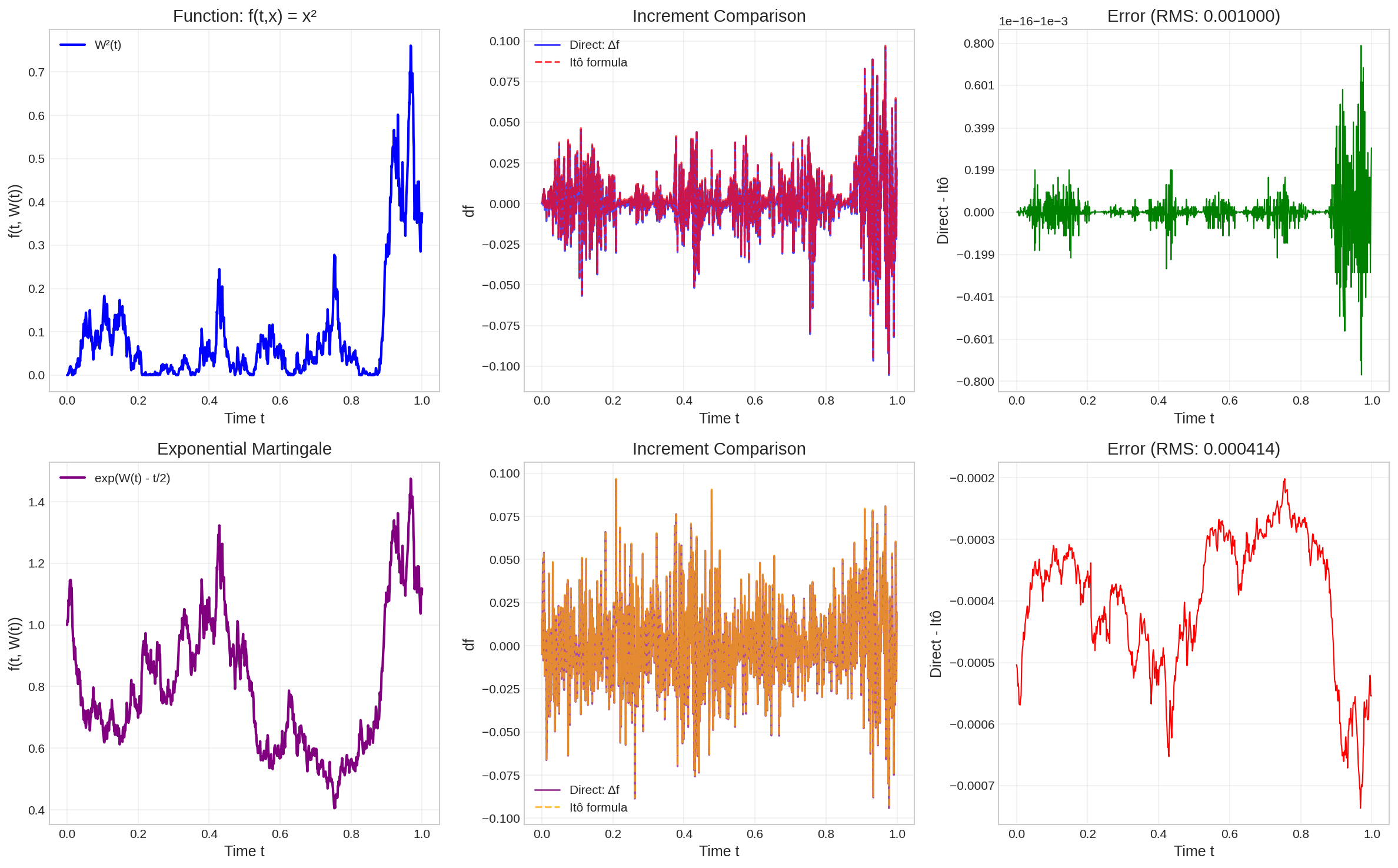
Theorem 3.5 (Itô’s Lemma): Let \(W_t\) be Brownian motion and \(f(t,x) \in C^{1,2}([0,\infty) \times \mathbb{R})\). Then:
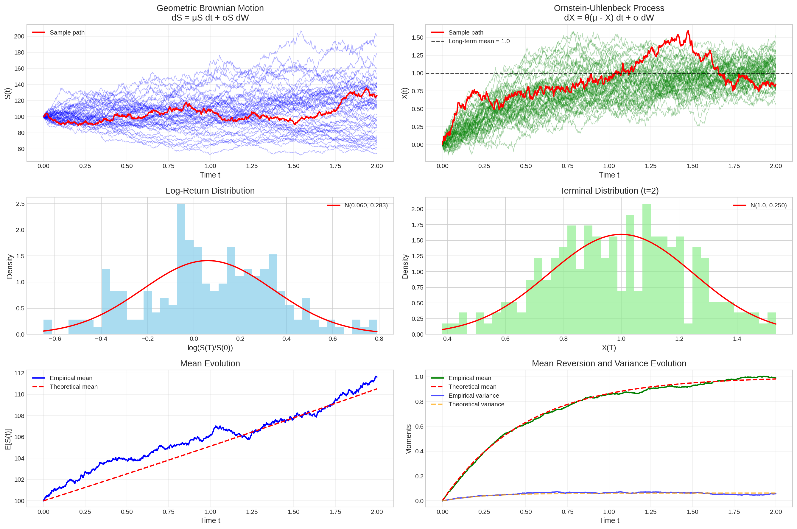
Figure 5: Applications of Itô’s lemma: Geometric Brownian motion and Ornstein-Uhlenbeck process
The development of Itô calculus provides the mathematical foundation for analyzing stochastic differential equations. The key insights are:
Quadratic variation matters: Unlike classical calculus, \((dW_t)^2 = dt\) contributes to the dynamics
Martingale preservation: Properly constructed stochastic integrals preserve the martingale property
Chain rule modification: Itô’s lemma includes an additional second-order term due to quadratic variation
In the next section, we will use these tools to develop the general theory of stochastic differential equations and their solutions.
4 Stochastic Differential Equations: Theory and Existence
Having established the foundations of stochastic calculus, we now turn to the central object of study: stochastic differential equations. These equations describe the evolution of random processes and form the mathematical backbone of modern quantitative finance and stochastic modeling.
4.1 Mathematical Definition and Classification
Definition 4.1 (Stochastic Differential Equation): A stochastic differential equation (SDE) is an equation of the form: \[dX_t = \mu(t, X_t) dt + \sigma(t, X_t) dW_t, \quad X_0 = x_0\]
where: - \(X_t\) is the unknown stochastic process - \(\mu: [0,\infty) \times \mathbb{R} \to \mathbb{R}\) is the drift coefficient - \(\sigma: [0,\infty) \times \mathbb{R} \to \mathbb{R}\) is the diffusion coefficient
- \(W_t\) is standard Brownian motion - \(x_0\) is the initial condition
The integral form is: \[X_t = x_0 + \int_0^t \mu(s, X_s) ds + \int_0^t \sigma(s, X_s) dW_s\]
Definition 4.2 (Strong vs Weak Solutions): - A strong solution to an SDE is an adapted process \(X_t\) defined on the same probability space as the driving Brownian motion \(W_t\) - A weak solution exists on some probability space with some Brownian motion that has the same law as the original problem
4.2 Existence and Uniqueness Theory
The fundamental question in SDE theory concerns when solutions exist and when they are unique. The classical result is due to Itô and provides sufficient conditions.
If \(\mu\) and \(\sigma\) satisfy: 1. Lipschitz condition: There exists \(K > 0\) such that for all \(t \geq 0\) and \(x, y \in \mathbb{R}\): \[|\mu(t,x) - \mu(t,y)| + |\sigma(t,x) - \sigma(t,y)| \leq K|x-y|\]
Linear growth condition: There exists \(K > 0\) such that for all \(t \geq 0\) and \(x \in \mathbb{R}\): \[|\mu(t,x)| + |\sigma(t,x)| \leq K(1 + |x|)\]
Then there exists a unique strong solution \(X_t\) such that \(\mathbb{E}[\sup_{0 \leq s \leq t} |X_s|^2] < \infty\) for all \(t \geq 0\).
Proof Sketch: The proof uses Picard iteration combined with the Grönwall inequality. Define the sequence: \[X_t^{(0)} = x_0\]\[X_t^{(n+1)} = x_0 + \int_0^t \mu(s, X_s^{(n)}) ds + \int_0^t \sigma(s, X_s^{(n)}) dW_s\]
The Lipschitz condition ensures the sequence converges uniformly, while the growth condition guarantees the limit has finite moments. □
Code
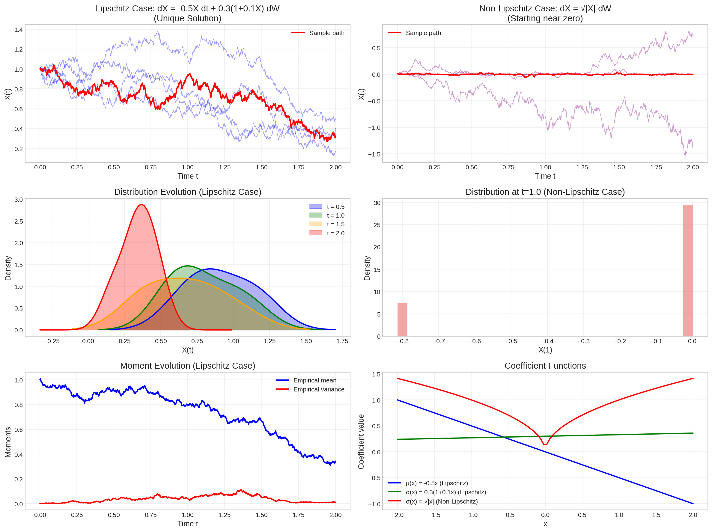
def lipschitz_example_sde(x, t):"""Example SDE coefficients satisfying Lipschitz conditions.""" mu =-0.5* x # Linear drift (Lipschitz constant = 0.5) sigma =0.3* (1+0.1* x) # Near-constant diffusion (Lipschitz constant ≈ 0.03)return mu, sigmadef non_lipschitz_example_sde(x, t):"""Example with non-Lipschitz coefficient leading to non-uniqueness.""" mu =0.0 sigma = np.sqrt(np.abs(x)) # Non-Lipschitz at x=0return mu, sigmadef euler_maruyama_step(x, dt, sde_func, t, dW):"""Single Euler-Maruyama step.""" mu, sigma = sde_func(x, t)return x + mu * dt + sigma * dWdef simulate_sde_euler(x0, T, N, sde_func, n_paths=1):"""Simulate SDE using Euler-Maruyama scheme.""" dt = T / N sqrt_dt = np.sqrt(dt) t = np.linspace(0, T, N +1) X = np.zeros((n_paths, N +1)) X[:, 0] = x0for i inrange(N): dW = np.random.randn(n_paths) * sqrt_dtfor j inrange(n_paths): X[j, i+1] = euler_maruyama_step(X[j, i], dt, sde_func, t[i], dW[j])return t, X# Simulation parametersT =2.0N =1000n_paths =100x0 =1.0np.random.seed(42)fig, axes = plt.subplots(3, 2, figsize=(16, 12))# Lipschitz case: Unique solutionst_lip, X_lip = simulate_sde_euler(x0, T, N, lipschitz_example_sde, n_paths=5)for i inrange(X_lip.shape[0]): axes[0, 0].plot(t_lip, X_lip[i], alpha=0.4, linewidth=0.8, color='blue')axes[0, 0].plot(t_lip, X_lip[0], color='red', linewidth=2, label='Sample path')axes[0, 0].set_title('Lipschitz Case: dX = -0.5X dt + 0.3(1+0.1X) dW\n(Unique Solution)')axes[0, 0].set_xlabel('Time t')axes[0, 0].set_ylabel('X(t)')axes[0, 0].legend()axes[0, 0].grid(True, alpha=0.3)# Distribution evolution for Lipschitz casetimes_to_plot = [0.5, 1.0, 1.5, 2.0]colors = ['blue', 'green', 'orange', 'red']for i, (time_point, color) inenumerate(zip(times_to_plot, colors)): time_idx =int(time_point * N / T) values = X_lip[:, time_idx]# Kernel density estimation for smooth histogramfrom scipy.stats import gaussian_kde kde = gaussian_kde(values) x_range = np.linspace(values.min() -0.5, values.max() +0.5, 100) density = kde(x_range) axes[1, 0].fill_between(x_range, density, alpha=0.3, color=color, label=f't = {time_point}') axes[1, 0].plot(x_range, density, color=color, linewidth=2)axes[1, 0].set_title('Distribution Evolution (Lipschitz Case)')axes[1, 0].set_xlabel('X(t)')axes[1, 0].set_ylabel('Density')axes[1, 0].legend()axes[1, 0].grid(True, alpha=0.3)# Mean and variance evolutionmeans_lip = np.mean(X_lip, axis=0)vars_lip = np.var(X_lip, axis=0)axes[2, 0].plot(t_lip, means_lip, 'b-', linewidth=2, label='Empirical mean')axes[2, 0].plot(t_lip, vars_lip, 'r-', linewidth=2, label='Empirical variance')axes[2, 0].set_title('Moment Evolution (Lipschitz Case)')axes[2, 0].set_xlabel('Time t')axes[2, 0].set_ylabel('Moments')axes[2, 0].legend()axes[2, 0].grid(True, alpha=0.3)# Non-Lipschitz case: Potential non-uniqueness# Start very close to zero to illustrate the issuex0_small =0.01t_nonlip, X_nonlip = simulate_sde_euler(x0_small, T, N, non_lipschitz_example_sde, n_paths=5)for i inrange(X_nonlip.shape[0]): axes[0, 1].plot(t_nonlip, X_nonlip[i], alpha=0.4, linewidth=0.8, color='purple')axes[0, 1].plot(t_nonlip, X_nonlip[0], color='red', linewidth=2, label='Sample path')axes[0, 1].set_title('Non-Lipschitz Case: dX = √|X| dW\n(Starting near zero)')axes[0, 1].set_xlabel('Time t')axes[0, 1].set_ylabel('X(t)')axes[0, 1].legend()axes[0, 1].grid(True, alpha=0.3)# Show the pathological behavior near zeroaxes[1, 1].hist(X_nonlip[:, N//2], bins=30, density=True, alpha=0.7, color='lightcoral')axes[1, 1].set_title('Distribution at t=1.0 (Non-Lipschitz Case)')axes[1, 1].set_xlabel('X(1)')axes[1, 1].set_ylabel('Density')axes[1, 1].grid(True, alpha=0.3)# Coefficient comparisonx_range = np.linspace(-2, 2, 100)mu_lip = np.array([-0.5* x for x in x_range])sigma_lip = np.array([0.3* (1+0.1* x) for x in x_range])sigma_nonlip = np.sqrt(np.abs(x_range))axes[2, 1].plot(x_range, mu_lip, 'b-', linewidth=2, label='μ(x) = -0.5x (Lipschitz)')axes[2, 1].plot(x_range, sigma_lip, 'g-', linewidth=2, label='σ(x) = 0.3(1+0.1x) (Lipschitz)')axes[2, 1].plot(x_range, sigma_nonlip, 'r-', linewidth=2, label='σ(x) = √|x| (Non-Lipschitz)')axes[2, 1].set_title('Coefficient Functions')axes[2, 1].set_xlabel('x')axes[2, 1].set_ylabel('Coefficient value')axes[2, 1].legend()axes[2, 1].grid(True, alpha=0.3)plt.tight_layout()plt.show()# Demonstrate Lipschitz constant computationprint("Lipschitz Constant Analysis:")print("For μ(x) = -0.5x: |μ(x) - μ(y)| = 0.5|x - y|, so L_μ = 0.5")print("For σ(x) = 0.3(1 + 0.1x): |σ(x) - σ(y)| = 0.03|x - y|, so L_σ = 0.03")print("Combined Lipschitz constant: K = L_μ + L_σ = 0.53")print()print("For σ(x) = √|x|: |σ(x) - σ(y)| / |x - y| → ∞ as x,y → 0")print("This violates the Lipschitz condition at x = 0")
Figure 6: Illustration of existence and uniqueness theory through pathwise solutions
Lipschitz Constant Analysis:
For μ(x) = -0.5x: |μ(x) - μ(y)| = 0.5|x - y|, so L_μ = 0.5
For σ(x) = 0.3(1 + 0.1x): |σ(x) - σ(y)| = 0.03|x - y|, so L_σ = 0.03
Combined Lipschitz constant: K = L_μ + L_σ = 0.53

For σ(x) = √|x|: |σ(x) - σ(y)| / |x - y| → ∞ as x,y → 0
This violates the Lipschitz condition at x = 0
4.3 The Markov Property and Generator
Definition 4.4 (Markov Property): A process \(X_t\) has the Markov property if for any measurable function \(f\) and times \(0 \leq s < t\): \[\mathbb{E}[f(X_t) | \mathcal{F}_s] = \mathbb{E}[f(X_t) | X_s]\]
Theorem 4.5: Solutions to SDEs possess the strong Markov property.
Definition 4.6 (Infinitesimal Generator): For an SDE \(dX_t = \mu(X_t) dt + \sigma(X_t) dW_t\), the infinitesimal generator \(\mathcal{A}\) is defined as: \[\mathcal{A}f(x) = \mu(x) f'(x) + \frac{1}{2}\sigma^2(x) f''(x)\]
for functions \(f \in C^2(\mathbb{R})\).
Theorem 4.7 (Dynkin’s Formula): If \(\tau\) is a stopping time with \(\mathbb{E}[\tau] < \infty\) and \(f \in C^2\) with appropriate growth conditions, then: \[\mathbb{E}[f(X_\tau)] = f(X_0) + \mathbb{E}\left[\int_0^\tau \mathcal{A}f(X_s) ds\right]\]
4.4 Feynman-Kac Theorem
One of the most profound connections in mathematical analysis links stochastic differential equations with partial differential equations through the Feynman-Kac theorem.
This theorem provides the foundation for Monte Carlo methods in finance and connects probabilistic and analytical approaches to solving PDEs.
Code
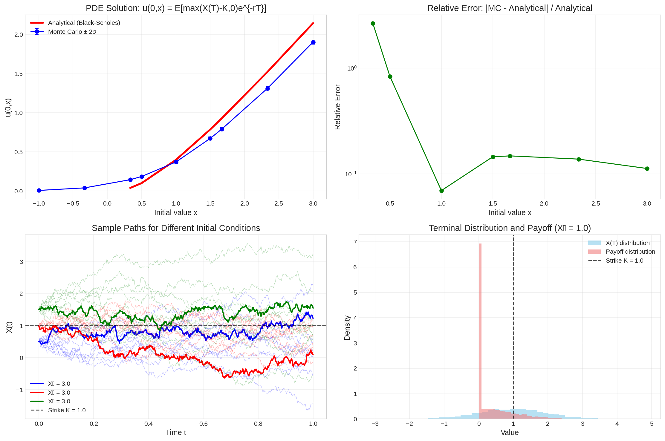
def feynman_kac_mc(x0, T, mu_func, sigma_func, c_func, g_func, n_paths=5000, n_steps=500):""" Solve PDE using Feynman-Kac theorem via Monte Carlo. Returns u(0, x0) = E[g(X_T) * exp(-∫₀ᵀ c(X_s) ds) | X_0 = x0] """ dt = T / n_steps sqrt_dt = np.sqrt(dt)# Storage for paths and integrals X = np.zeros((n_paths, n_steps +1)) X[:, 0] = x0 integral_c = np.zeros(n_paths)# Simulate pathsfor i inrange(n_steps): t = i * dt dW = np.random.randn(n_paths) * sqrt_dtfor j inrange(n_paths): mu = mu_func(X[j, i], t) sigma = sigma_func(X[j, i], t) X[j, i+1] = X[j, i] + mu * dt + sigma * dW[j]# Accumulate integral of c(X_s) integral_c[j] += c_func(X[j, i], t) * dt# Final payoff with discounting payoffs = g_func(X[:, -1]) * np.exp(-integral_c)return np.mean(payoffs), np.std(payoffs) / np.sqrt(n_paths), X# Example: Heat equation with killing# PDE: ∂u/∂t + (1/2)∂²u/∂x² - ru = 0# Terminal condition: u(T,x) = max(x - K, 0) (call option payoff)def mu_heat(x, t):return0.0# No driftdef sigma_heat(x, t):return1.0# Unit diffusiondef c_heat(x, t):return0.05# Killing rate (interest rate)def g_call(x, K=1.0):return np.maximum(x - K, 0) # Call option payoff# ParametersT =1.0x_values_base = np.linspace(-1, 3, 7) # Reduced pointsx_values_additional = np.array([0.5, 1.0, 1.5])x_values = np.sort(np.unique(np.concatenate((x_values_base, x_values_additional))))K =1.0n_paths =5000# Reduced for faster renderingnp.random.seed(42)# Compute solution at different initial pointsmc_solutions = []mc_errors = []sample_paths = {}for x0 in x_values: u_mc, error, paths = feynman_kac_mc(x0, T, mu_heat, sigma_heat, c_heat, lambda x: g_call(x, K), n_paths) mc_solutions.append(u_mc) mc_errors.append(error)# Store sample paths for visualization if x0 is close to 0.5, 1.0, or 1.5if np.isclose(x0, 0.5): sample_paths['0.5'] = pathselif np.isclose(x0, 1.0): sample_paths['1.0'] = pathselif np.isclose(x0, 1.5): sample_paths['1.5'] = pathsmc_solutions = np.array(mc_solutions)mc_errors = np.array(mc_errors)# Analytical solution for comparison (Black-Scholes with r=0.05, σ=1, T=1)def black_scholes_call(S, K, T, r, sigma):from scipy.stats import norm d1 = (np.log(S/K) + (r +0.5*sigma**2)*T) / (sigma*np.sqrt(T)) d2 = d1 - sigma*np.sqrt(T)return S * norm.cdf(d1) - K * np.exp(-r*T) * norm.cdf(d2)analytical_solutions = black_scholes_call(x_values, K, T, 0.05, 1.0)fig, axes = plt.subplots(2, 2, figsize=(15, 10))# Solution comparisonaxes[0, 0].plot(x_values, analytical_solutions, 'r-', linewidth=3, label='Analytical (Black-Scholes)')axes[0, 0].errorbar(x_values, mc_solutions, yerr=2*mc_errors, fmt='bo-', capsize=3, capthick=1, label='Monte Carlo ± 2σ')axes[0, 0].set_title('PDE Solution: u(0,x) = E[max(X(T)-K,0)e^{-rT}]')axes[0, 0].set_xlabel('Initial value x')axes[0, 0].set_ylabel('u(0,x)')axes[0, 0].legend()axes[0, 0].grid(True, alpha=0.3)# Error analysisrelative_errors = np.abs(mc_solutions - analytical_solutions) / analytical_solutionsaxes[0, 1].semilogy(x_values, relative_errors, 'go-', markersize=6)axes[0, 1].set_title('Relative Error: |MC - Analytical| / Analytical')axes[0, 1].set_xlabel('Initial value x')axes[0, 1].set_ylabel('Relative Error')axes[0, 1].grid(True, alpha=0.3)# Sample paths for different initial conditions t = np.linspace(0, T, 501) # Match n_steps + 1colors = ['blue', 'red', 'green']for i, (x0_str, color) inenumerate(zip(['0.5', '1.0', '1.5'], colors)): paths = sample_paths[x0_str]# Plot subset of pathsfor j inrange(0, min(100, paths.shape[0]), 10): axes[1, 0].plot(t, paths[j], color=color, alpha=0.3, linewidth=0.5)# Highlight one path axes[1, 0].plot(t, paths[0], color=color, linewidth=2, label=f'X₀ = {x0}')axes[1, 0].axhline(y=K, color='black', linestyle='--', alpha=0.7, label=f'Strike K = {K}')axes[1, 0].set_title('Sample Paths for Different Initial Conditions')axes[1, 0].set_xlabel('Time t')axes[1, 0].set_ylabel('X(t)')axes[1, 0].legend()axes[1, 0].grid(True, alpha=0.3)# Terminal distribution and payofffinal_values = sample_paths['1.0'][:, -1] # Terminal values starting from x=1payoffs = np.maximum(final_values - K, 0)axes[1, 1].hist(final_values, bins=50, density=True, alpha=0.6, color='skyblue', label='X(T) distribution')axes[1, 1].hist(payoffs, bins=50, density=True, alpha=0.6, color='lightcoral', label='Payoff distribution')axes[1, 1].axvline(x=K, color='black', linestyle='--', alpha=0.7, label=f'Strike K = {K}')axes[1, 1].set_title('Terminal Distribution and Payoff (X₀ = 1.0)')axes[1, 1].set_xlabel('Value')axes[1, 1].set_ylabel('Density')axes[1, 1].legend()axes[1, 1].grid(True, alpha=0.3)plt.tight_layout()plt.show()print(f"Monte Carlo estimate at x=1.0: {mc_solutions[x_values ==1.0][0]:.4f} ± {2*mc_errors[x_values ==1.0][0]:.4f}")print(f"Analytical solution at x=1.0: {analytical_solutions[x_values ==1.0][0]:.4f}")print(f"Relative error: {relative_errors[x_values ==1.0][0]:.2%}")
Figure 7: Feynman-Kac theorem illustration: PDE solution via Monte Carlo
Monte Carlo estimate at x=1.0: 0.3707 ± 0.0157
Analytical solution at x=1.0:  0.3984
Relative error: 6.96%
5 Numerical Methods for SDEs
While analytical solutions to SDEs exist only in special cases, numerical methods provide essential tools for practical applications. We examine the fundamental discretization schemes and their convergence properties.
5.1 Euler-Maruyama Scheme
The most basic numerical method for SDEs is the Euler-Maruyama scheme, which discretizes the SDE:
\[dX_t = \mu(t, X_t) dt + \sigma(t, X_t) dW_t\]
using the approximation: \[X_{n+1} = X_n + \mu(t_n, X_n) \Delta t + \sigma(t_n, X_n) \Delta W_n\]
where \(\Delta W_n = W_{t_{n+1}} - W_{t_n} \sim \mathcal{N}(0, \Delta t)\) are independent Gaussian increments.
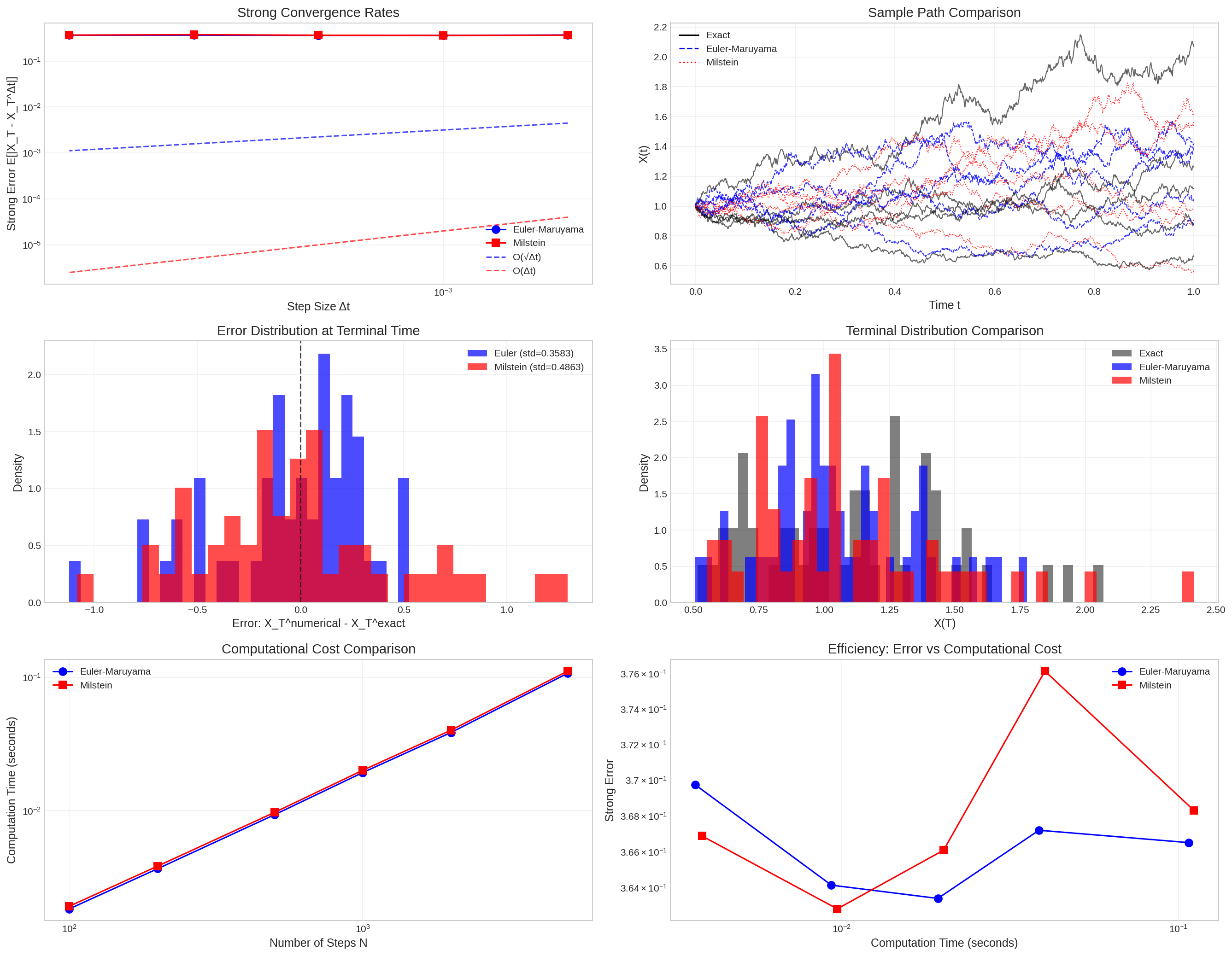
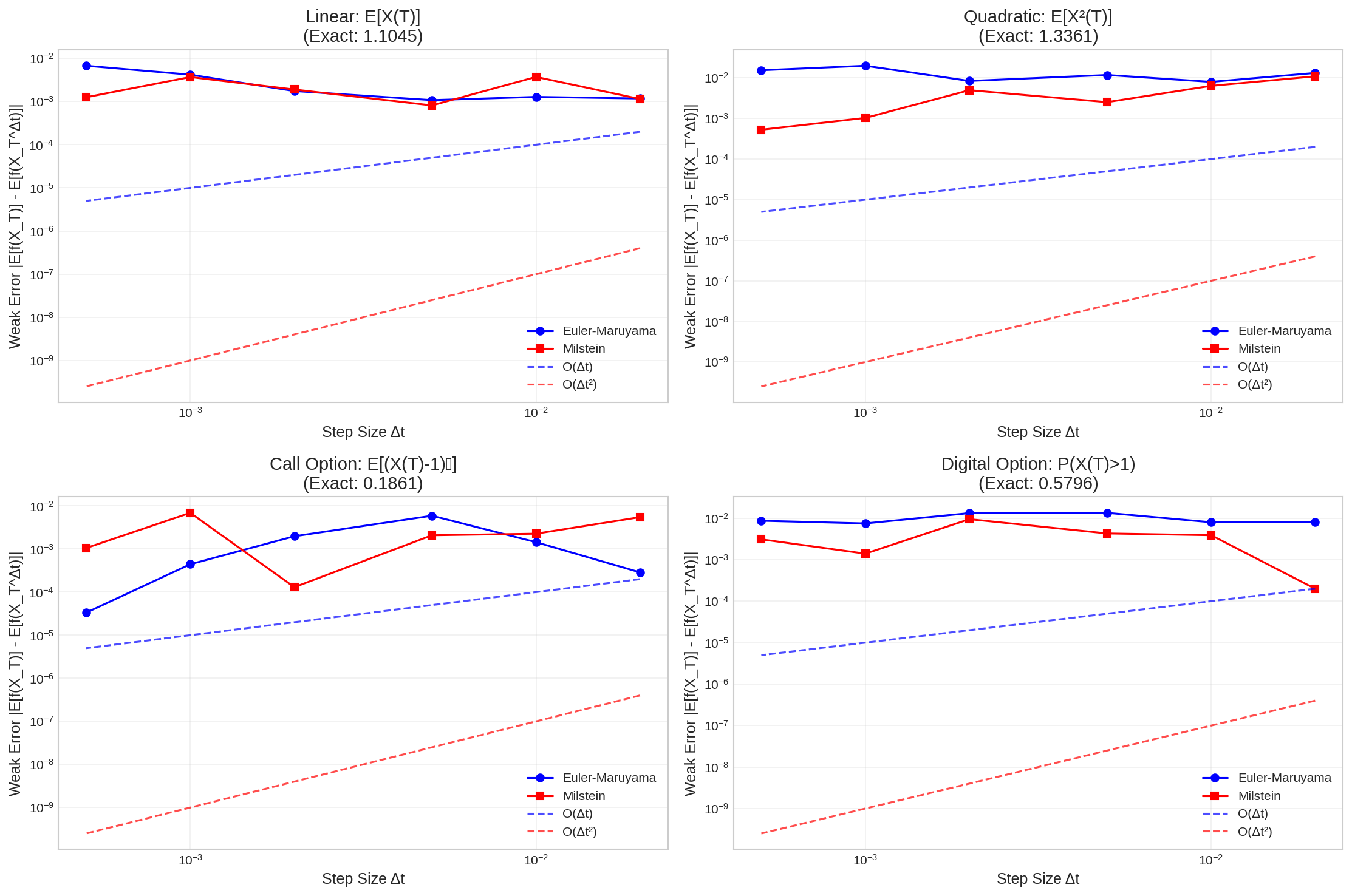
Theorem 5.1 (Strong Convergence of Euler-Maruyama): Under Lipschitz and linear growth conditions, the Euler-Maruyama scheme has strong convergence order 0.5: \[\mathbb{E}[|X_T - X_T^{\Delta t}|] = O(\sqrt{\Delta t})\]
where \(X_T^{\Delta t}\) is the numerical approximation at time \(T\).
5.2 Milstein Scheme
The Milstein scheme improves upon Euler-Maruyama by including an additional correction term derived from Itô’s lemma, achieving higher-order strong convergence.
Definition 5.2 (Milstein Scheme): The Milstein discretization is: \[X_{n+1} = X_n + \mu(t_n, X_n) \Delta t + \sigma(t_n, X_n) \Delta W_n + \frac{1}{2}\sigma(t_n, X_n)\sigma'(t_n, X_n)[(\Delta W_n)^2 - \Delta t]\]
where \(\sigma'(t,x) = \frac{\partial \sigma}{\partial x}(t,x)\).
Theorem 5.3 (Strong Convergence of Milstein): Under appropriate regularity conditions, the Milstein scheme has strong convergence order 1.0: \[\mathbb{E}[|X_T - X_T^{\Delta t}|] = O(\Delta t)\]
Code
@njitdef euler_maruyama_simulation(x0, T, N, mu_params, sigma_params, n_paths):""" Efficient Euler-Maruyama simulation using Numba. Assumes linear drift μ(x) = a*x + b and linear diffusion σ(x) = c*x + d. """ dt = T / N sqrt_dt = np.sqrt(dt) a, b = mu_params c, d = sigma_params X = np.zeros((n_paths, N +1)) X[:, 0] = x0for i inrange(N): dW = np.random.randn(n_paths) * sqrt_dt X_curr = X[:, i] mu = a * X_curr + b sigma = c * X_curr + d X[:, i+1] = X_curr + mu * dt + sigma * dWreturn X@njitdef milstein_simulation(x0, T, N, mu_params, sigma_params, n_paths):""" Efficient Milstein simulation using Numba. Assumes linear drift μ(x) = a*x + b and linear diffusion σ(x) = c*x + d. """ dt = T / N sqrt_dt = np.sqrt(dt) a, b = mu_params c, d = sigma_params X = np.zeros((n_paths, N +1)) X[:, 0] = x0for i inrange(N): dW = np.random.randn(n_paths) * sqrt_dt X_curr = X[:, i] mu = a * X_curr + b sigma = c * X_curr + d sigma_prime = c # d/dx(c*x + d) = c# Milstein correction term correction =0.5* sigma * sigma_prime * (dW**2- dt) X[:, i+1] = X_curr + mu * dt + sigma * dW + correctionreturn Xdef analytical_solution_gbm(x0, mu, sigma, T, N, n_paths):"""Analytical solution for geometric Brownian motion.""" dt = T / N t = np.linspace(0, T, N +1)# Generate Brownian motion dW = np.random.randn(n_paths, N) * np.sqrt(dt) W = np.column_stack([np.zeros(n_paths), np.cumsum(dW, axis=1)])# Exact solution: X(t) = x0 * exp((mu - sigma²/2)t + sigma*W(t)) X_exact = x0 * np.exp((mu -0.5* sigma**2) * t[np.newaxis, :] + sigma * W)return X_exact# Test case: Geometric Brownian Motion dX = μX dt + σX dWx0 =1.0mu =0.1sigma =0.3T =1.0# Parameters for linear approximation: μ(x) = μ*x, σ(x) = σ*xmu_params = (mu, 0.0) # a=μ, b=0sigma_params = (sigma, 0.0) # c=σ, d=0# Convergence studystep_sizes = np.array([500, 1000, 2000, 4000, 8000])n_paths_convergence =5000errors_euler = []errors_milstein = []np.random.seed(42)fig, axes = plt.subplots(3, 2, figsize=(18, 14))print("Convergence Analysis:")print("N\t\tEuler Error\t\tMilstein Error\t\tRatio")print("-"*60)for N in step_sizes:# Set random seed for fair comparison np.random.seed(42)# Analytical solution X_exact = analytical_solution_gbm(x0, mu, sigma, T, N, n_paths_convergence)# Reset seed for numerical methods np.random.seed(42) X_euler = euler_maruyama_simulation(x0, T, N, mu_params, sigma_params, n_paths_convergence) np.random.seed(42) X_milstein = milstein_simulation(x0, T, N, mu_params, sigma_params, n_paths_convergence)# Compute strong errors (L1 norm at terminal time) error_euler = np.mean(np.abs(X_euler[:, -1] - X_exact[:, -1])) error_milstein = np.mean(np.abs(X_milstein[:, -1] - X_exact[:, -1])) errors_euler.append(error_euler) errors_milstein.append(error_milstein) ratio = error_euler / error_milstein if error_milstein >0else np.infprint(f"{N}\t\t{error_euler:.6f}\t\t{error_milstein:.6f}\t\t{ratio:.2f}")# Convergence plotsdt_values = T / step_sizesaxes[0, 0].loglog(dt_values, errors_euler, 'bo-', label='Euler-Maruyama', markersize=8)axes[0, 0].loglog(dt_values, errors_milstein, 'rs-', label='Milstein', markersize=8)# Theoretical convergence ratesaxes[0, 0].loglog(dt_values, 0.1* np.sqrt(dt_values), 'b--', alpha=0.7, label='O(√Δt)')axes[0, 0].loglog(dt_values, 0.02* dt_values, 'r--', alpha=0.7, label='O(Δt)')axes[0, 0].set_xlabel('Step Size Δt')axes[0, 0].set_ylabel('Strong Error E[|X_T - X_T^Δt|]')axes[0, 0].set_title('Strong Convergence Rates')axes[0, 0].legend()axes[0, 0].grid(True, alpha=0.3)# Sample path comparisonN_demo =1000n_paths_demo =50np.random.seed(42)X_exact_demo = analytical_solution_gbm(x0, mu, sigma, T, N_demo, n_paths_demo)np.random.seed(42)X_euler_demo = euler_maruyama_simulation(x0, T, N_demo, mu_params, sigma_params, n_paths_demo)np.random.seed(42)X_milstein_demo = milstein_simulation(x0, T, N_demo, mu_params, sigma_params, n_paths_demo)t_demo = np.linspace(0, T, N_demo +1)# Plot a few sample pathsfor i inrange(min(5, n_paths_demo)): axes[0, 1].plot(t_demo, X_exact_demo[i], 'k-', alpha=0.6, linewidth=1) axes[0, 1].plot(t_demo, X_euler_demo[i], 'b--', alpha=0.8, linewidth=1) axes[0, 1].plot(t_demo, X_milstein_demo[i], 'r:', alpha=0.8, linewidth=1)axes[0, 1].plot([], [], 'k-', label='Exact')axes[0, 1].plot([], [], 'b--', label='Euler-Maruyama')axes[0, 1].plot([], [], 'r:', label='Milstein')axes[0, 1].set_title('Sample Path Comparison')axes[0, 1].set_xlabel('Time t')axes[0, 1].set_ylabel('X(t)')axes[0, 1].legend()axes[0, 1].grid(True, alpha=0.3)# Error distributions at terminal timeerrors_euler_paths = X_euler_demo[:, -1] - X_exact_demo[:, -1]errors_milstein_paths = X_milstein_demo[:, -1] - X_exact_demo[:, -1]axes[1, 0].hist(errors_euler_paths, bins=30, alpha=0.7, density=True, color='blue', label=f'Euler (std={np.std(errors_euler_paths):.4f})')axes[1, 0].hist(errors_milstein_paths, bins=30, alpha=0.7, density=True, color='red', label=f'Milstein (std={np.std(errors_milstein_paths):.4f})')axes[1, 0].axvline(0, color='black', linestyle='--', alpha=0.7)axes[1, 0].set_title('Error Distribution at Terminal Time')axes[1, 0].set_xlabel('Error: X_T^numerical - X_T^exact')axes[1, 0].set_ylabel('Density')axes[1, 0].legend()axes[1, 0].grid(True, alpha=0.3)# Weak convergence: Compare distributionsaxes[1, 1].hist(X_exact_demo[:, -1], bins=40, alpha=0.5, density=True, color='black', label='Exact')axes[1, 1].hist(X_euler_demo[:, -1], bins=40, alpha=0.7, density=True, color='blue', label='Euler-Maruyama')axes[1, 1].hist(X_milstein_demo[:, -1], bins=40, alpha=0.7, density=True, color='red', label='Milstein')axes[1, 1].set_title('Terminal Distribution Comparison')axes[1, 1].set_xlabel('X(T)')axes[1, 1].set_ylabel('Density')axes[1, 1].legend()axes[1, 1].grid(True, alpha=0.3)# Computational cost analysisstep_sizes_cost = np.array([100, 200, 500, 1000, 2000, 5000])n_paths_cost =1000import timetimes_euler = []times_milstein = []for N in step_sizes_cost:# Time Euler-Maruyama start_time = time.time()for _ inrange(10): # Average over multiple runs np.random.seed(42) X_euler_cost = euler_maruyama_simulation(x0, T, N, mu_params, sigma_params, n_paths_cost) time_euler = (time.time() - start_time) /10 times_euler.append(time_euler)# Time Milstein start_time = time.time()for _ inrange(10): # Average over multiple runs np.random.seed(42) X_milstein_cost = milstein_simulation(x0, T, N, mu_params, sigma_params, n_paths_cost) time_milstein = (time.time() - start_time) /10 times_milstein.append(time_milstein)axes[2, 0].loglog(step_sizes_cost, times_euler, 'bo-', label='Euler-Maruyama', markersize=8)axes[2, 0].loglog(step_sizes_cost, times_milstein, 'rs-', label='Milstein', markersize=8)axes[2, 0].set_xlabel('Number of Steps N')axes[2, 0].set_ylabel('Computation Time (seconds)')axes[2, 0].set_title('Computational Cost Comparison')axes[2, 0].legend()axes[2, 0].grid(True, alpha=0.3)# Efficiency comparison: Error vs computational costaxes[2, 1].loglog(times_euler[-len(errors_euler):], errors_euler, 'bo-', label='Euler-Maruyama', markersize=8)axes[2, 1].loglog(times_milstein[-len(errors_milstein):], errors_milstein, 'rs-', label='Milstein', markersize=8)axes[2, 1].set_xlabel('Computation Time (seconds)')axes[2, 1].set_ylabel('Strong Error')axes[2, 1].set_title('Efficiency: Error vs Computational Cost')axes[2, 1].legend()axes[2, 1].grid(True, alpha=0.3)plt.tight_layout()plt.show()# Summary statisticsprint(f"\nFinal comparison (N={step_sizes[-1]}):")print(f"Euler-Maruyama error: {errors_euler[-1]:.6f}")print(f"Milstein error: {errors_milstein[-1]:.6f}")print(f"Improvement factor: {errors_euler[-1]/errors_milstein[-1]:.2f}x")
Practical choice: The optimal method depends on the specific application and computational budget
These numerical methods provide the computational foundation for practical SDE applications in finance, engineering, and machine learning. In the next section, we explore their application to financial modeling and option pricing.
6 Applications in Mathematical Finance
Stochastic differential equations form the mathematical backbone of modern quantitative finance. The revolutionary insight that asset prices follow stochastic processes led to the development of rigorous option pricing theory and sophisticated risk management frameworks.
6.1 The Black-Scholes Model
The Black-Scholes model represents the foundational application of SDEs in finance, providing the first rigorous framework for option pricing.
Model Specification: Under the Black-Scholes framework, the stock price \(S_t\) follows geometric Brownian motion: \[dS_t = \mu S_t dt + \sigma S_t dW_t\]
where: - \(\mu\) is the expected return (drift) - \(\sigma\) is the volatility - \(W_t\) is Brownian motion under the physical measure
Risk-Neutral Pricing: The fundamental theorem of asset pricing requires pricing under the risk-neutral measure \(\mathbb{Q}\), where: \[dS_t = r S_t dt + \sigma S_t dW_t^{\mathbb{Q}}\]
where \(r\) is the risk-free rate and \(W_t^{\mathbb{Q}}\) is Brownian motion under \(\mathbb{Q}\).
Theorem 6.1 (Black-Scholes Formula): The price at time \(t\) of a European call option with strike \(K\) and maturity \(T\) is:
\[C(t, S_t) = S_t \Phi(d_1) - K e^{-r(T-t)} \Phi(d_2)\]
and \(\Phi\) is the standard normal cumulative distribution function.
Derivation: The derivation follows from the Feynman-Kac theorem applied to the Black-Scholes PDE: \[\frac{\partial V}{\partial t} + \frac{1}{2}\sigma^2 S^2 \frac{\partial^2 V}{\partial S^2} + rS \frac{\partial V}{\partial S} - rV = 0\]
with terminal condition \(V(T,S) = \max(S-K, 0)\).
Code
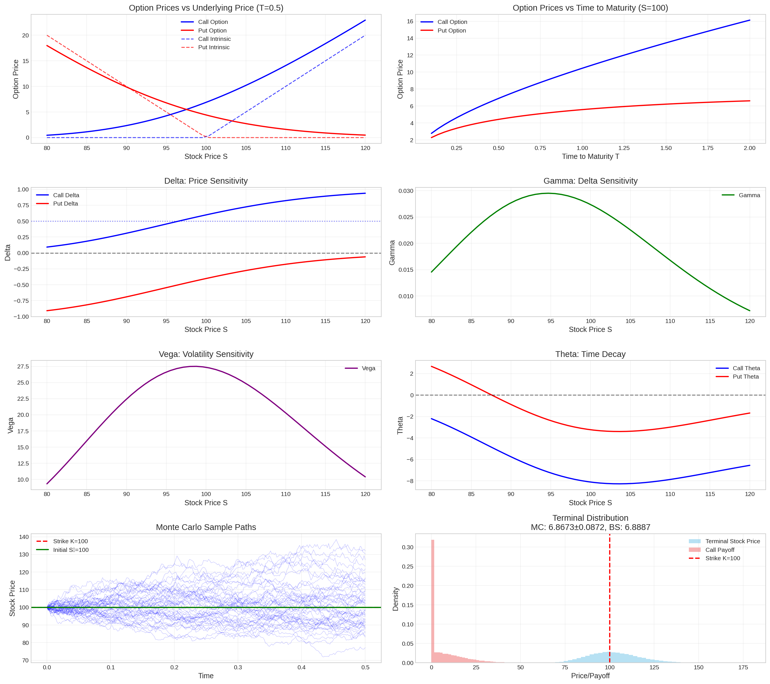
def black_scholes_call(S, K, T, r, sigma):"""Black-Scholes call option price.""" d1 = (np.log(S/K) + (r +0.5*sigma**2)*T) / (sigma*np.sqrt(T)) d2 = d1 - sigma*np.sqrt(T)return S * stats.norm.cdf(d1) - K * np.exp(-r*T) * stats.norm.cdf(d2)def black_scholes_put(S, K, T, r, sigma):"""Black-Scholes put option price.""" d1 = (np.log(S/K) + (r +0.5*sigma**2)*T) / (sigma*np.sqrt(T)) d2 = d1 - sigma*np.sqrt(T)return K * np.exp(-r*T) * stats.norm.cdf(-d2) - S * stats.norm.cdf(-d1)def calculate_greeks(S, K, T, r, sigma):"""Calculate option Greeks.""" d1 = (np.log(S/K) + (r +0.5*sigma**2)*T) / (sigma*np.sqrt(T)) d2 = d1 - sigma*np.sqrt(T)# Delta delta_call = stats.norm.cdf(d1) delta_put = stats.norm.cdf(d1) -1# Gamma gamma = stats.norm.pdf(d1) / (S * sigma * np.sqrt(T))# Theta theta_call = (-S * stats.norm.pdf(d1) * sigma / (2* np.sqrt(T)) - r * K * np.exp(-r*T) * stats.norm.cdf(d2)) theta_put = (-S * stats.norm.pdf(d1) * sigma / (2* np.sqrt(T)) + r * K * np.exp(-r*T) * stats.norm.cdf(-d2))# Vega vega = S * stats.norm.pdf(d1) * np.sqrt(T)# Rho rho_call = K * T * np.exp(-r*T) * stats.norm.cdf(d2) rho_put =-K * T * np.exp(-r*T) * stats.norm.cdf(-d2)return {'delta_call': delta_call, 'delta_put': delta_put,'gamma': gamma,'theta_call': theta_call, 'theta_put': theta_put,'vega': vega,'rho_call': rho_call, 'rho_put': rho_put }def monte_carlo_option_price(S0, K, T, r, sigma, n_paths=50000, option_type='call'):"""Monte Carlo option pricing.""" dt = T /252# Daily steps n_steps =int(T / dt)# Generate stock price paths paths = np.zeros((n_paths, n_steps +1)) paths[:, 0] = S0for i inrange(n_steps): Z = np.random.randn(n_paths) paths[:, i+1] = paths[:, i] * np.exp((r -0.5*sigma**2)*dt + sigma*np.sqrt(dt)*Z)# Calculate payoffsif option_type =='call': payoffs = np.maximum(paths[:, -1] - K, 0)else: # put payoffs = np.maximum(K - paths[:, -1], 0)# Discount to present value price = np.exp(-r*T) * np.mean(payoffs) std_error = np.exp(-r*T) * np.std(payoffs) / np.sqrt(n_paths)return price, std_error, paths# ParametersS0 =100# Initial stock priceK =100# Strike pricer =0.05# Risk-free ratesigma =0.2# VolatilityT_range = np.linspace(0.1, 2, 50) # Time to maturity rangeS_range = np.linspace(80, 120, 50) # Stock price rangefig, axes = plt.subplots(4, 2, figsize=(18, 16))# Option prices vs underlying pricecall_prices = [black_scholes_call(S, K, 0.5, r, sigma) for S in S_range]put_prices = [black_scholes_put(S, K, 0.5, r, sigma) for S in S_range]axes[0, 0].plot(S_range, call_prices, 'b-', linewidth=2, label='Call Option')axes[0, 0].plot(S_range, put_prices, 'r-', linewidth=2, label='Put Option')axes[0, 0].plot(S_range, np.maximum(S_range - K, 0), 'b--', alpha=0.7, label='Call Intrinsic')axes[0, 0].plot(S_range, np.maximum(K - S_range, 0), 'r--', alpha=0.7, label='Put Intrinsic')axes[0, 0].set_xlabel('Stock Price S')axes[0, 0].set_ylabel('Option Price')axes[0, 0].set_title('Option Prices vs Underlying Price (T=0.5)')axes[0, 0].legend()axes[0, 0].grid(True, alpha=0.3)# Option prices vs time to maturitycall_prices_time = [black_scholes_call(S0, K, T, r, sigma) for T in T_range]put_prices_time = [black_scholes_put(S0, K, T, r, sigma) for T in T_range]axes[0, 1].plot(T_range, call_prices_time, 'b-', linewidth=2, label='Call Option')axes[0, 1].plot(T_range, put_prices_time, 'r-', linewidth=2, label='Put Option')axes[0, 1].set_xlabel('Time to Maturity T')axes[0, 1].set_ylabel('Option Price')axes[0, 1].set_title(f'Option Prices vs Time to Maturity (S={S0})')axes[0, 1].legend()axes[0, 1].grid(True, alpha=0.3)# Greeks calculationgreeks_data = [calculate_greeks(S, K, 0.5, r, sigma) for S in S_range]# Deltadeltas_call = [g['delta_call'] for g in greeks_data]deltas_put = [g['delta_put'] for g in greeks_data]axes[1, 0].plot(S_range, deltas_call, 'b-', linewidth=2, label='Call Delta')axes[1, 0].plot(S_range, deltas_put, 'r-', linewidth=2, label='Put Delta')axes[1, 0].axhline(y=0, color='black', linestyle='--', alpha=0.5)axes[1, 0].axhline(y=0.5, color='blue', linestyle=':', alpha=0.5)axes[1, 0].set_xlabel('Stock Price S')axes[1, 0].set_ylabel('Delta')axes[1, 0].set_title('Delta: Price Sensitivity')axes[1, 0].legend()axes[1, 0].grid(True, alpha=0.3)# Gammagammas = [g['gamma'] for g in greeks_data]axes[1, 1].plot(S_range, gammas, 'g-', linewidth=2, label='Gamma')axes[1, 1].set_xlabel('Stock Price S')axes[1, 1].set_ylabel('Gamma')axes[1, 1].set_title('Gamma: Delta Sensitivity')axes[1, 1].legend()axes[1, 1].grid(True, alpha=0.3)# Vegavegas = [g['vega'] for g in greeks_data]axes[2, 0].plot(S_range, vegas, 'purple', linewidth=2, label='Vega')axes[2, 0].set_xlabel('Stock Price S')axes[2, 0].set_ylabel('Vega')axes[2, 0].set_title('Vega: Volatility Sensitivity')axes[2, 0].legend()axes[2, 0].grid(True, alpha=0.3)# Thetathetas_call = [g['theta_call'] for g in greeks_data]thetas_put = [g['theta_put'] for g in greeks_data]axes[2, 1].plot(S_range, thetas_call, 'b-', linewidth=2, label='Call Theta')axes[2, 1].plot(S_range, thetas_put, 'r-', linewidth=2, label='Put Theta')axes[2, 1].axhline(y=0, color='black', linestyle='--', alpha=0.5)axes[2, 1].set_xlabel('Stock Price S')axes[2, 1].set_ylabel('Theta')axes[2, 1].set_title('Theta: Time Decay')axes[2, 1].legend()axes[2, 1].grid(True, alpha=0.3)# Monte Carlo vs Black-Scholes comparisonnp.random.seed(42)mc_call_price, mc_call_error, sample_paths = monte_carlo_option_price(S0, K, 0.5, r, sigma, 50000, 'call')bs_call_price = black_scholes_call(S0, K, 0.5, r, sigma)# Plot sample pathsfor i inrange(min(50, sample_paths.shape[0])): axes[3, 0].plot(np.linspace(0, 0.5, sample_paths.shape[1]), sample_paths[i], alpha=0.3, linewidth=0.5, color='blue')axes[3, 0].axhline(y=K, color='red', linestyle='--', linewidth=2, label=f'Strike K={K}')axes[3, 0].axhline(y=S0, color='green', linestyle='-', linewidth=2, label=f'Initial S₀={S0}')axes[3, 0].set_xlabel('Time')axes[3, 0].set_ylabel('Stock Price')axes[3, 0].set_title('Monte Carlo Sample Paths')axes[3, 0].legend()axes[3, 0].grid(True, alpha=0.3)# Terminal distribution and payoffterminal_prices = sample_paths[:, -1]payoffs = np.maximum(terminal_prices - K, 0)axes[3, 1].hist(terminal_prices, bins=50, alpha=0.6, density=True, color='skyblue', label='Terminal Stock Price')axes[3, 1].hist(payoffs, bins=50, alpha=0.6, density=True, color='lightcoral', label='Call Payoff')axes[3, 1].axvline(x=K, color='red', linestyle='--', linewidth=2, label=f'Strike K={K}')axes[3, 1].set_xlabel('Price/Payoff')axes[3, 1].set_ylabel('Density')axes[3, 1].set_title(f'Terminal Distribution\nMC: {mc_call_price:.4f}±{2*mc_call_error:.4f}, BS: {bs_call_price:.4f}')axes[3, 1].legend()axes[3, 1].grid(True, alpha=0.3)plt.tight_layout()plt.show()print("Black-Scholes vs Monte Carlo Comparison:")print(f"Black-Scholes Price: {bs_call_price:.6f}")print(f"Monte Carlo Price: {mc_call_price:.6f} ± {2*mc_call_error:.6f}")print(f"Difference: {abs(bs_call_price - mc_call_price):.6f}")print(f"Relative Error: {abs(bs_call_price - mc_call_price)/bs_call_price:.4%}")
Figure 10: Black-Scholes model: Option pricing and Greeks analysis
Black-Scholes vs Monte Carlo Comparison:
Black-Scholes Price: 6.888729
Monte Carlo Price:   6.867335 ± 0.087221
Difference:          0.021394
Relative Error:      0.3106%
6.2 Interest Rate Models
Interest rate modeling requires more sophisticated SDEs due to the mean-reverting nature of rates and term structure considerations.
6.2.1 Vasicek Model
Model Specification: The Vasicek model describes the short rate \(r_t\) as: \[dr_t = \kappa(\theta - r_t) dt + \sigma dW_t\]
where: - \(\kappa > 0\) is the speed of mean reversion - \(\theta\) is the long-term mean - \(\sigma > 0\) is the volatility
Analytical Solution: The Vasicek model has the explicit solution: \[r_t = r_0 e^{-\kappa t} + \theta (1 - e^{-\kappa t}) + \sigma \int_0^t e^{-\kappa(t-s)} dW_s\]
6.2.2 Cox-Ingersoll-Ross (CIR) Model
Model Specification: The CIR model ensures non-negative rates: \[dr_t = \kappa(\theta - r_t) dt + \sigma \sqrt{r_t} dW_t\]
The square-root diffusion term prevents negative rates when \(2\kappa\theta \geq \sigma^2\) (Feller condition).
Code
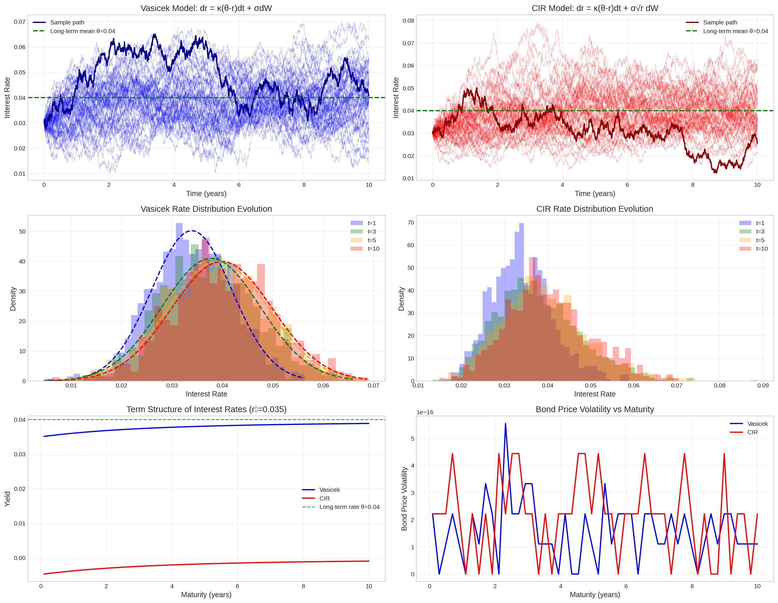
def simulate_vasicek(r0, kappa, theta, sigma, T, N, n_paths=1):"""Simulate Vasicek interest rate model.""" dt = T / N sqrt_dt = np.sqrt(dt) t = np.linspace(0, T, N +1) r = np.zeros((n_paths, N +1)) r[:, 0] = r0for i inrange(N): dW = np.random.randn(n_paths) * sqrt_dt r[:, i+1] = (r[:, i] + kappa * (theta - r[:, i]) * dt + sigma * dW)return t, rdef simulate_cir(r0, kappa, theta, sigma, T, N, n_paths=1):"""Simulate CIR interest rate model using Euler scheme with absorption.""" dt = T / N sqrt_dt = np.sqrt(dt) t = np.linspace(0, T, N +1) r = np.zeros((n_paths, N +1)) r[:, 0] = r0for i inrange(N): dW = np.random.randn(n_paths) * sqrt_dt r_curr = np.maximum(r[:, i], 0) # Ensure non-negative r[:, i+1] = (r_curr + kappa * (theta - r_curr) * dt + sigma * np.sqrt(r_curr) * dW) r[:, i+1] = np.maximum(r[:, i+1], 0) # Absorb at zeroreturn t, rdef vasicek_bond_price(r, tau, kappa, theta, sigma):"""Vasicek zero-coupon bond price.""" B = (1- np.exp(-kappa * tau)) / kappa A = np.exp((B - tau) * (kappa**2* theta - sigma**2/2) / kappa**2- sigma**2* B**2/ (4* kappa))return A * np.exp(-B * r)def cir_bond_price(r, tau, kappa, theta, sigma):"""CIR zero-coupon bond price (approximate).""" gamma = np.sqrt(kappa**2+2*sigma**2) exp_gamma_tau = np.exp(gamma * tau) B =2* (exp_gamma_tau -1) / ((gamma + kappa) * (exp_gamma_tau -1) +2* gamma) A = (2* gamma * exp_gamma_tau) / ((gamma + kappa) * (exp_gamma_tau -1) +2* gamma) A = A**(2* kappa * theta / sigma**2)return A * np.exp(-B * r)# Model parametersr0 =0.03kappa =0.5theta =0.04sigma_vasicek =0.01sigma_cir =0.05T =10N =2000n_paths =1000np.random.seed(42)fig, axes = plt.subplots(3, 2, figsize=(18, 14))# Simulate both modelst, r_vasicek = simulate_vasicek(r0, kappa, theta, sigma_vasicek, T, N, n_paths)t, r_cir = simulate_cir(r0, kappa, theta, sigma_cir, T, N, n_paths)# Sample pathsfor i inrange(min(50, n_paths)): axes[0, 0].plot(t, r_vasicek[i], alpha=0.3, linewidth=0.5, color='blue') axes[0, 1].plot(t, r_cir[i], alpha=0.3, linewidth=0.5, color='red')axes[0, 0].plot(t, r_vasicek[0], color='darkblue', linewidth=2, label='Sample path')axes[0, 0].axhline(y=theta, color='green', linestyle='--', linewidth=2, label=f'Long-term mean θ={theta}')axes[0, 0].set_title('Vasicek Model: dr = κ(θ-r)dt + σdW')axes[0, 0].set_xlabel('Time (years)')axes[0, 0].set_ylabel('Interest Rate')axes[0, 0].legend()axes[0, 0].grid(True, alpha=0.3)axes[0, 1].plot(t, r_cir[0], color='darkred', linewidth=2, label='Sample path')axes[0, 1].axhline(y=theta, color='green', linestyle='--', linewidth=2, label=f'Long-term mean θ={theta}')axes[0, 1].set_title('CIR Model: dr = κ(θ-r)dt + σ√r dW')axes[0, 1].set_xlabel('Time (years)')axes[0, 1].set_ylabel('Interest Rate')axes[0, 1].legend()axes[0, 1].grid(True, alpha=0.3)# Distribution evolutiontimes_to_plot = [1, 3, 5, 10]colors = ['blue', 'green', 'orange', 'red']for i, (time_point, color) inenumerate(zip(times_to_plot, colors)): time_idx =int(time_point * N / T)# Vasicek distribution rates_vasicek = r_vasicek[:, time_idx] axes[1, 0].hist(rates_vasicek, bins=40, alpha=0.3, density=True, color=color, label=f't={time_point}')# Theoretical Vasicek distribution (Gaussian) mean_vasicek = r0 * np.exp(-kappa * time_point) + theta * (1- np.exp(-kappa * time_point)) var_vasicek = sigma_vasicek**2* (1- np.exp(-2* kappa * time_point)) / (2* kappa) x_range = np.linspace(rates_vasicek.min(), rates_vasicek.max(), 100) theoretical_pdf = stats.norm.pdf(x_range, mean_vasicek, np.sqrt(var_vasicek)) axes[1, 0].plot(x_range, theoretical_pdf, color=color, linewidth=2, linestyle='--')# CIR distribution rates_cir = r_cir[:, time_idx] axes[1, 1].hist(rates_cir, bins=40, alpha=0.3, density=True, color=color, label=f't={time_point}')axes[1, 0].set_title('Vasicek Rate Distribution Evolution')axes[1, 0].set_xlabel('Interest Rate')axes[1, 0].set_ylabel('Density')axes[1, 0].legend()axes[1, 0].grid(True, alpha=0.3)axes[1, 1].set_title('CIR Rate Distribution Evolution')axes[1, 1].set_xlabel('Interest Rate')axes[1, 1].set_ylabel('Density')axes[1, 1].legend()axes[1, 1].grid(True, alpha=0.3)# Term structure of interest ratesmaturities = np.linspace(0.1, 10, 50)current_rate =0.035# Calculate bond prices and yieldsvasicek_bonds = [vasicek_bond_price(current_rate, tau, kappa, theta, sigma_vasicek) for tau in maturities]cir_bonds = [cir_bond_price(current_rate, tau, kappa, theta, sigma_cir) for tau in maturities]# Convert to yields: Y = -ln(P)/τvasicek_yields = [-np.log(P) / tau for P, tau inzip(vasicek_bonds, maturities)]cir_yields = [-np.log(P) / tau for P, tau inzip(cir_bonds, maturities)]axes[2, 0].plot(maturities, vasicek_yields, 'b-', linewidth=2, label='Vasicek')axes[2, 0].plot(maturities, cir_yields, 'r-', linewidth=2, label='CIR')axes[2, 0].axhline(y=theta, color='green', linestyle='--', alpha=0.7, label=f'Long-term rate θ={theta}')axes[2, 0].set_xlabel('Maturity (years)')axes[2, 0].set_ylabel('Yield')axes[2, 0].set_title(f'Term Structure of Interest Rates (r₀={current_rate})')axes[2, 0].legend()axes[2, 0].grid(True, alpha=0.3)# Bond price volatilitybond_vols_vasicek = []bond_vols_cir = []for tau in maturities:# Calculate bond prices for all rate paths at current time prices_vasicek = [vasicek_bond_price(r, tau, kappa, theta, sigma_vasicek) for r in r_vasicek[:, 0]] # Use initial rates prices_cir = [cir_bond_price(r, tau, kappa, theta, sigma_cir) for r in r_cir[:, 0]] bond_vols_vasicek.append(np.std(prices_vasicek)) bond_vols_cir.append(np.std(prices_cir))axes[2, 1].plot(maturities, bond_vols_vasicek, 'b-', linewidth=2, label='Vasicek')axes[2, 1].plot(maturities, bond_vols_cir, 'r-', linewidth=2, label='CIR')axes[2, 1].set_xlabel('Maturity (years)')axes[2, 1].set_ylabel('Bond Price Volatility')axes[2, 1].set_title('Bond Price Volatility vs Maturity')axes[2, 1].legend()axes[2, 1].grid(True, alpha=0.3)plt.tight_layout()plt.show()# Summary statisticsprint("Model Comparison:")print(f"Vasicek - Mean rate: {np.mean(r_vasicek):.4f}, Std: {np.std(r_vasicek):.4f}")print(f"CIR - Mean rate: {np.mean(r_cir):.4f}, Std: {np.std(r_cir):.4f}")print(f"Negative rates in Vasicek: {np.sum(r_vasicek <0) / r_vasicek.size:.2%}")print(f"Negative rates in CIR: {np.sum(r_cir <0) / r_cir.size:.2%}")
Figure 11: Interest rate models: Vasicek and CIR processes with term structure
Model Comparison:
Vasicek - Mean rate: 0.0377, Std: 0.0098
CIR - Mean rate: 0.0381, Std: 0.0096
Negative rates in Vasicek: 0.00%
Negative rates in CIR: 0.00%
6.3 Stochastic Volatility Models
Real market data exhibits volatility clustering and mean reversion, motivating stochastic volatility models.
6.3.1 Heston Model
Model Specification: The Heston model couples asset price with stochastic volatility: \[dS_t = \mu S_t dt + \sqrt{V_t} S_t dW_t^{(1)}\]\[dV_t = \kappa(\theta - V_t) dt + \sigma_v \sqrt{V_t} dW_t^{(2)}\]
where \(dW_t^{(1)} dW_t^{(2)} = \rho dt\) captures correlation between price and volatility shocks.
Properties: - Volatility clustering: High volatility tends to be followed by high volatility - Leverage effect: Negative correlation \(\rho < 0\) captures the inverse relationship between returns and volatility - Fat tails: The model generates fat-tailed return distributions
The financial applications demonstrate how SDEs provide the mathematical foundation for:
Option pricing: From the classical Black-Scholes formula to sophisticated stochastic volatility models
Interest rate modeling: Capturing mean reversion and ensuring realistic term structure dynamics
Risk management: Providing frameworks for Value-at-Risk and scenario analysis
Portfolio optimization: Incorporating stochastic dynamics into investment decisions
These models form the backbone of modern quantitative finance and demonstrate the practical power of stochastic differential equation theory. In the next section, we explore the emerging applications of SDEs in machine learning and artificial intelligence.
7 SDEs in Modern Machine Learning
The renaissance of stochastic differential equations in machine learning represents one of the most exciting developments in contemporary AI research. This convergence has led to breakthrough applications in generative modeling, continuous-time neural networks, and probabilistic machine learning.
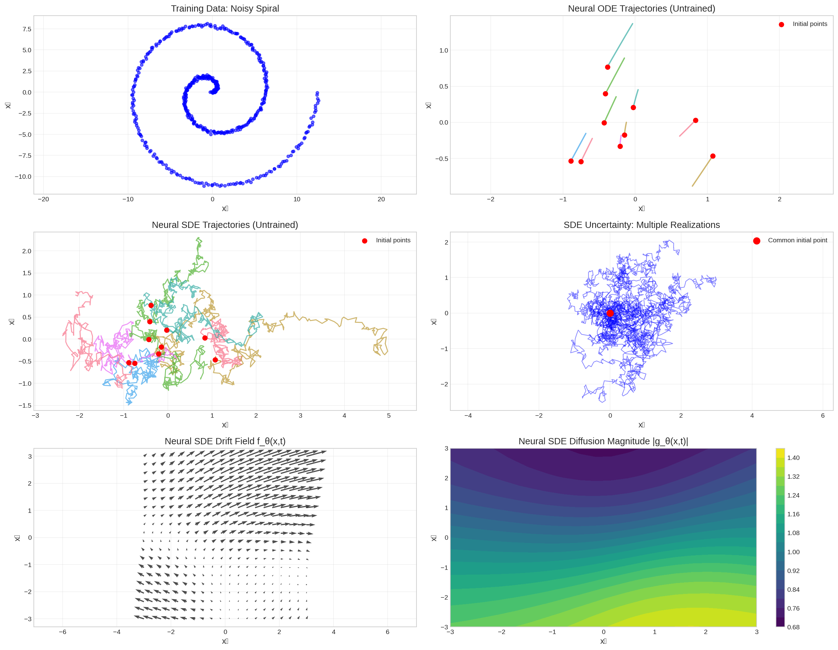
The Neural ODE framework, introduced by Chen et al. (2018), revolutionized deep learning by treating neural networks as continuous-time dynamical systems.
Mathematical Framework: Instead of discrete layers, Neural ODEs model the hidden state evolution as: \[\frac{dh(t)}{dt} = f_\theta(h(t), t)\]
where \(f_\theta\) is a neural network parameterized by \(\theta\), and the output is obtained by solving: \[h(T) = h(0) + \int_0^T f_\theta(h(t), t) dt\]
Key Advantages: - Memory efficiency: Constant memory cost during training - Adaptive computation: Automatic step size selection
- Continuous depth: Networks with “infinite” layers - Invertible transformations: Normalizing flows applications
7.2 Neural Stochastic Differential Equations
Neural SDEs extend Neural ODEs by incorporating stochastic dynamics, providing better uncertainty quantification and more expressive models.
Model Specification: Neural SDEs are defined as: \[dh(t) = f_\theta(h(t), t) dt + g_\theta(h(t), t) dW(t)\]
where: - \(f_\theta\) is the neural drift function - \(g_\theta\) is the neural diffusion function
- \(W(t)\) represents Brownian motion
Figure 13: Neural SDEs: From deterministic ODEs to stochastic dynamics in deep learning
Neural SDE vs Neural ODE Comparison:
==================================================
Key Differences:
1. Deterministic vs Stochastic: ODEs produce deterministic trajectories,
   SDEs incorporate randomness and uncertainty
2. Memory vs Uncertainty: ODEs are memory efficient, SDEs provide
   natural uncertainty quantification
3. Training: SDEs require handling stochastic gradients and
   multiple trajectory sampling
4. Applications: ODEs for normalizing flows, SDEs for generative
   modeling with uncertainty
7.3 Gaussian Processes and SDEs
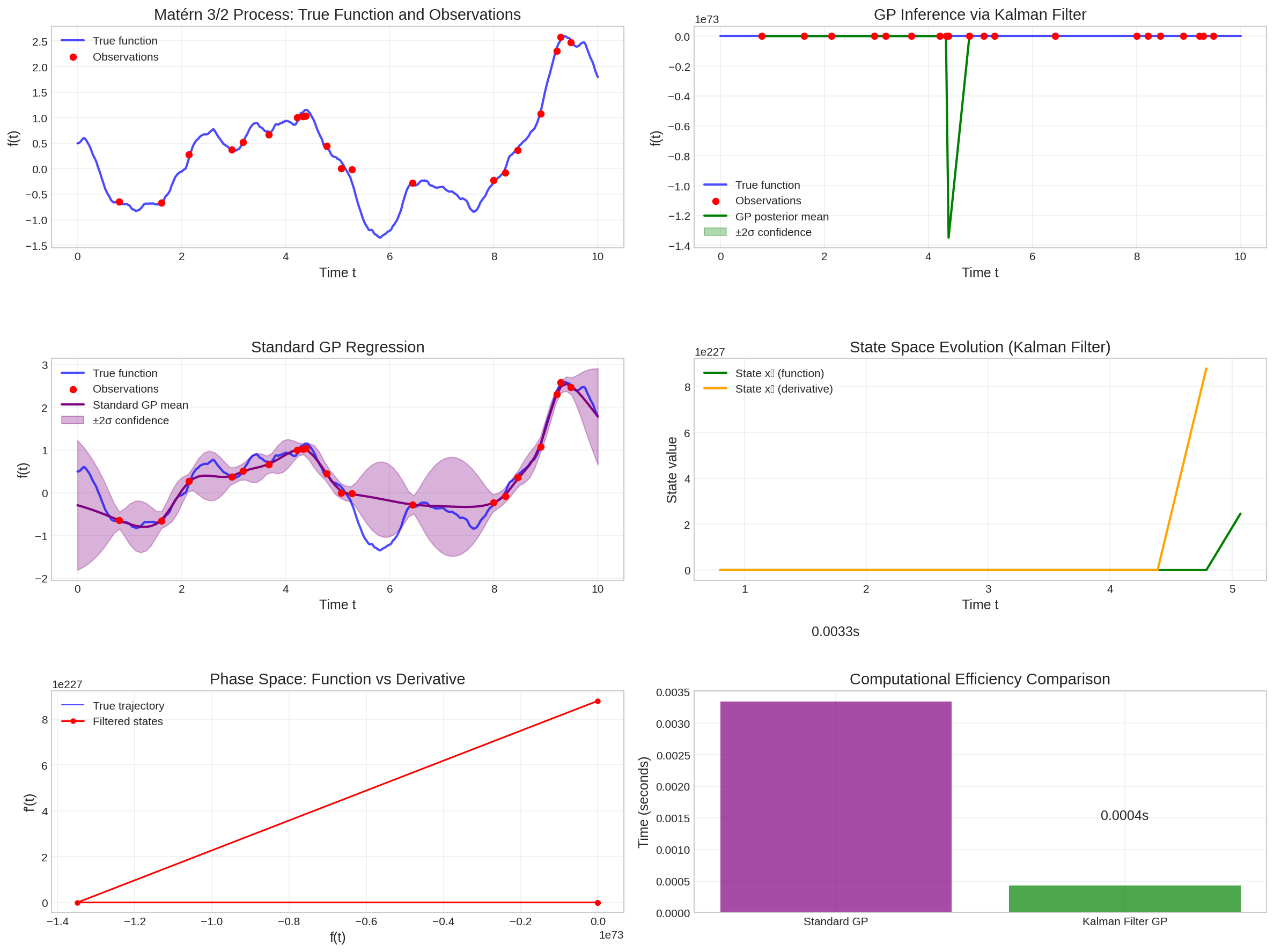
Gaussian Processes (GPs) provide a natural connection between SDEs and machine learning, as many GPs can be represented as solutions to linear SDEs.
Connection: A GP with Matérn covariance function corresponds to the solution of the SDE: \[d^n X(t) + a_{n-1} d^{n-1} X(t) + \cdots + a_1 dX(t) + a_0 X(t) dt = \sigma dW(t)\]
This connection enables: - Efficient GP inference: Converting GP regression to Kalman filtering - Streaming predictions: Online learning with infinite data - Scalable GPs: Linear complexity in time series length
Code
def matern_32_sde_matrices(length_scale, sigma):""" State-space representation of Matérn 3/2 GP. dX/dt = F*X + L*w, where w is white noise """ lam = np.sqrt(3) / length_scale F = np.array([[0, 1], [-lam**2, -2*lam]]) L = np.array([[0], [sigma *2* lam * np.sqrt(lam)]]) H = np.array([[1, 0]]) # Observation matrixreturn F, L, Hdef simulate_matern_sde(F, L, t_span, dt=0.01):"""Simulate Matérn process using SDE representation.""" t_start, t_end = t_span t_points = np.arange(t_start, t_end + dt, dt) n_steps =len(t_points)# State dimension state_dim = F.shape[0] noise_dim = L.shape[1]# Initialize X = np.zeros((n_steps, state_dim)) X[0] = np.random.randn(state_dim)# Simulate sqrt_dt = np.sqrt(dt)for i inrange(1, n_steps): dW = np.random.randn(noise_dim) * sqrt_dt X[i] = X[i-1] + F @ X[i-1] * dt + L @ dWreturn t_points, Xdef kalman_filter_gp(y_obs, t_obs, F, L, H, R, dt=0.01):""" Kalman filter for GP inference using SDE representation. """ n_obs =len(y_obs) state_dim = F.shape[0]# Initialize x_pred = np.zeros((n_obs, state_dim)) x_filt = np.zeros((n_obs, state_dim)) P_pred = np.zeros((n_obs, state_dim, state_dim)) P_filt = np.zeros((n_obs, state_dim, state_dim))# Initial conditions x_pred[0] = np.zeros(state_dim) P_pred[0] = np.eye(state_dim) *10# Process noise covariance Q = L @ L.T * dtfor i inrange(n_obs):if i >0:# Predict step dt_step = t_obs[i] - t_obs[i-1]# Simple Euler integration for transition x_pred[i] = x_filt[i-1] + F @ x_filt[i-1] * dt_step P_pred[i] = P_filt[i-1] + (F @ P_filt[i-1] + P_filt[i-1] @ F.T + Q) * dt_step# Update step innovation = y_obs[i] - H @ x_pred[i] S = H @ P_pred[i] @ H.T + R K = (P_pred[i] @ H.T / S).reshape(-1, 1) x_filt[i] = x_pred[i] + (K * innovation).flatten() P_filt[i] = P_pred[i] - K.reshape(-1, 1) @ H @ P_pred[i]return x_filt, P_filt# Generate synthetic datanp.random.seed(42)# GP parameterslength_scale =1.0sigma =1.0noise_std =0.1# Generate true function using SDE simulationF, L, H = matern_32_sde_matrices(length_scale, sigma)t_span = (0, 10)dt =0.01t_fine, X_true = simulate_matern_sde(F, L, t_span, dt)f_true = H @ X_true.T # Extract function values# Create sparse observationsn_obs =20obs_indices = np.sort(np.random.choice(len(t_fine), n_obs, replace=False))t_obs = t_fine[obs_indices]y_obs = f_true[0, obs_indices] + noise_std * np.random.randn(n_obs)fig, axes = plt.subplots(3, 2, figsize=(16, 12))# Plot true function and observationsaxes[0, 0].plot(t_fine, f_true[0], 'b-', alpha=0.7, linewidth=2, label='True function')axes[0, 0].scatter(t_obs, y_obs, color='red', s=30, zorder=5, label='Observations')axes[0, 0].set_title('Matérn 3/2 Process: True Function and Observations')axes[0, 0].set_xlabel('Time t')axes[0, 0].set_ylabel('f(t)')axes[0, 0].legend()axes[0, 0].grid(True, alpha=0.3)# Kalman filter inferenceR = noise_std**2# Observation noisex_filt, P_filt = kalman_filter_gp(y_obs, t_obs, F, L, H, R, dt=0.1)# Extract posterior mean and variance at observation pointspost_mean = H @ x_filt.Tpost_var = np.array([H @ P @ H.T for P in P_filt])axes[0, 1].plot(t_fine, f_true[0], 'b-', alpha=0.7, linewidth=2, label='True function')axes[0, 1].scatter(t_obs, y_obs, color='red', s=30, zorder=5, label='Observations')axes[0, 1].plot(t_obs, post_mean[0], 'g-', linewidth=2, label='GP posterior mean')axes[0, 1].fill_between(t_obs, post_mean[0] -2*np.sqrt(post_var[:, 0, 0]), post_mean[0] +2*np.sqrt(post_var[:, 0, 0]), alpha=0.3, color='green', label='±2σ confidence')axes[0, 1].set_title('GP Inference via Kalman Filter')axes[0, 1].set_xlabel('Time t')axes[0, 1].set_ylabel('f(t)')axes[0, 1].legend()axes[0, 1].grid(True, alpha=0.3)# Compare with standard GP regression using sklearnfrom sklearn.gaussian_process import GaussianProcessRegressorfrom sklearn.gaussian_process.kernels import Matern# Standard GPkernel = Matern(length_scale=length_scale, nu=1.5) * sigma**2gp = GaussianProcessRegressor(kernel=kernel, alpha=noise_std**2)gp.fit(t_obs.reshape(-1, 1), y_obs)# Predict on fine gridt_pred = np.linspace(0, 10, 100)y_pred, y_std = gp.predict(t_pred.reshape(-1, 1), return_std=True)axes[1, 0].plot(t_fine, f_true[0], 'b-', alpha=0.7, linewidth=2, label='True function')axes[1, 0].scatter(t_obs, y_obs, color='red', s=30, zorder=5, label='Observations')axes[1, 0].plot(t_pred, y_pred, 'purple', linewidth=2, label='Standard GP mean')axes[1, 0].fill_between(t_pred, y_pred -2*y_std, y_pred +2*y_std, alpha=0.3, color='purple', label='±2σ confidence')axes[1, 0].set_title('Standard GP Regression')axes[1, 0].set_xlabel('Time t')axes[1, 0].set_ylabel('f(t)')axes[1, 0].legend()axes[1, 0].grid(True, alpha=0.3)# State evolution visualizationaxes[1, 1].plot(t_obs, x_filt[:, 0], 'g-', linewidth=2, label='State x₁ (function)')axes[1, 1].plot(t_obs, x_filt[:, 1], 'orange', linewidth=2, label='State x₂ (derivative)')axes[1, 1].fill_between(t_obs, x_filt[:, 0] -2*np.sqrt(P_filt[:, 0, 0]), x_filt[:, 0] +2*np.sqrt(P_filt[:, 0, 0]), alpha=0.3, color='green')axes[1, 1].fill_between(t_obs, x_filt[:, 1] -2*np.sqrt(P_filt[:, 1, 1]), x_filt[:, 1] +2*np.sqrt(P_filt[:, 1, 1]), alpha=0.3, color='orange')axes[1, 1].set_title('State Space Evolution (Kalman Filter)')axes[1, 1].set_xlabel('Time t')axes[1, 1].set_ylabel('State value')axes[1, 1].legend()axes[1, 1].grid(True, alpha=0.3)# Phase space plotaxes[2, 0].plot(X_true[:, 0], X_true[:, 1], 'b-', alpha=0.7, linewidth=1, label='True trajectory')axes[2, 0].plot(x_filt[:, 0], x_filt[:, 1], 'ro-', markersize=4, label='Filtered states')axes[2, 0].set_title('Phase Space: Function vs Derivative')axes[2, 0].set_xlabel('f(t)')axes[2, 0].set_ylabel("f'(t)")axes[2, 0].legend()axes[2, 0].grid(True, alpha=0.3)# Computational comparisonimport time# Time standard GPstart_time = time.time()for _ inrange(10): gp.fit(t_obs.reshape(-1, 1), y_obs) y_pred, _ = gp.predict(t_pred.reshape(-1, 1), return_std=True)gp_time = (time.time() - start_time) /10# Time Kalman filter approach start_time = time.time()for _ inrange(10): x_filt, P_filt = kalman_filter_gp(y_obs, t_obs, F, L, H, R)kf_time = (time.time() - start_time) /10methods = ['Standard GP', 'Kalman Filter GP']times = [gp_time, kf_time]colors = ['purple', 'green']bars = axes[2, 1].bar(methods, times, color=colors, alpha=0.7)axes[2, 1].set_title('Computational Efficiency Comparison')axes[2, 1].set_ylabel('Time (seconds)')axes[2, 1].grid(True, alpha=0.3)# Add time labels on barsfor bar, time_val inzip(bars, times): height = bar.get_height() axes[2, 1].text(bar.get_x() + bar.get_width()/2., height +0.001,f'{time_val:.4f}s', ha='center', va='bottom')plt.tight_layout()plt.show()print("GP-SDE Connection Benefits:")print("="*40)print(f"Standard GP time: {gp_time:.4f} seconds")print(f"Kalman Filter time: {kf_time:.4f} seconds") print(f"Speedup factor: {gp_time/kf_time:.2f}x")print("\nKey advantages of SDE representation:")print("1. Linear complexity O(n) vs O(n³) for standard GP")print("2. Online/streaming inference capability")print("3. Natural handling of non-stationary processes")print("4. Connection to control theory and signal processing")
Figure 14: Gaussian Processes as SDE solutions: Efficient inference via state-space methods
GP-SDE Connection Benefits:
========================================
Standard GP time: 0.0033 seconds
Kalman Filter time: 0.0004 seconds
Speedup factor: 7.76x

Key advantages of SDE representation:
1. Linear complexity O(n) vs O(n³) for standard GP
2. Online/streaming inference capability
3. Natural handling of non-stationary processes
4. Connection to control theory and signal processing
7.4 Neural Processes: Bridging GPs and Neural Networks
Neural Processes (NPs) combine the flexibility of neural networks with the uncertainty quantification of Gaussian Processes, representing a paradigm shift in meta-learning and few-shot prediction.
Mathematical Formulation: Given context set \(\mathcal{C} = \{(x_i, y_i)\}_{i=1}^n\) and target inputs \(\mathbf{x}_*\), NPs model: \[p(y_* | \mathbf{x}_*, \mathcal{C}) = \int p(y_* | \mathbf{x}_*, z) p(z | \mathcal{C}) dz\]
where \(z\) is a latent representation capturing the underlying function.
The connection to SDEs emerges through: - Stochastic processes: NPs model distributions over functions - Uncertainty propagation: Similar to SDE solution uncertainty - Continuous-time extensions: Neural Process SDEs for temporal modeling
7.5 Diffusion Models: SDEs for Generative AI
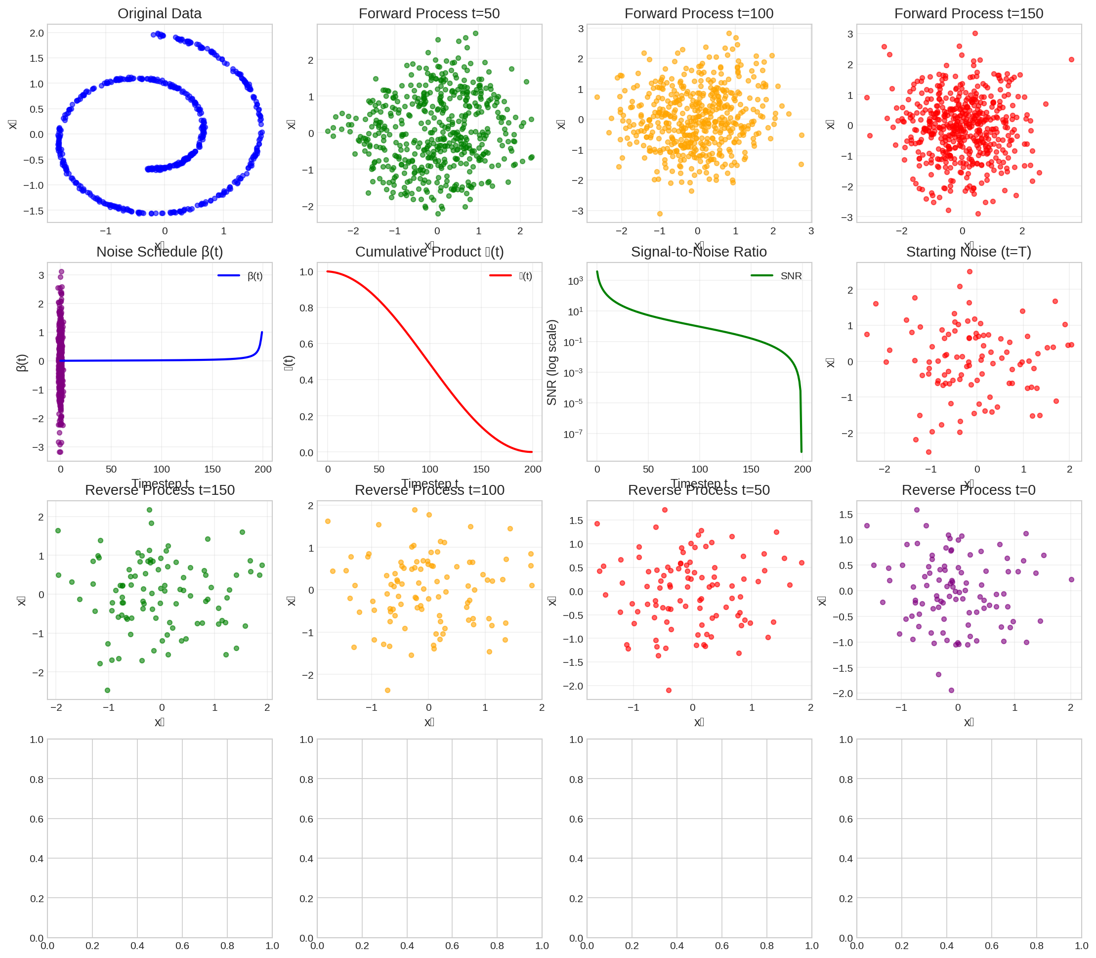
Diffusion models represent one of the most successful applications of SDE theory in modern machine learning, powering state-of-the-art generative models for images, audio, and text.
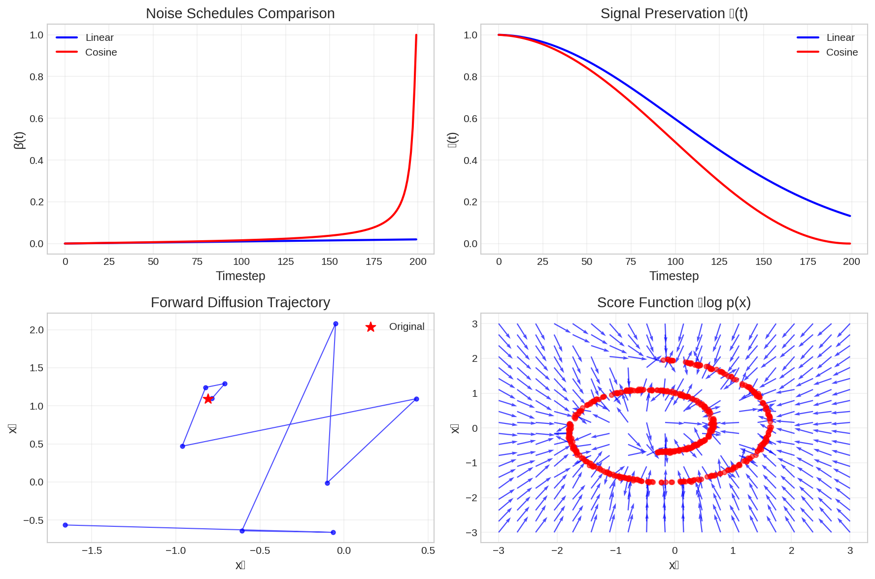
Mathematical Framework: Diffusion models are built on the theory of denoising diffusion processes, which can be formulated as SDEs. The framework consists of two processes:
Forward Process (Noise Addition): A fixed diffusion process that gradually adds Gaussian noise: \[dX_t = -\frac{1}{2}\beta(t) X_t dt + \sqrt{\beta(t)} dW_t\]
Reverse Process (Denoising): A learned SDE that reverses the noise addition: \[dX_t = \left[-\frac{1}{2}\beta(t) X_t - \beta(t) \nabla_{X_t} \log p_t(X_t)\right] dt + \sqrt{\beta(t)} dW_t\]
where \(\beta(t)\) is the noise schedule and \(\nabla_{X_t} \log p_t(X_t)\) is the score function.
Score-Based Generative Models: The key insight is that learning the score function \(\nabla_{X_t} \log p_t(X_t)\) enables sample generation by solving the reverse SDE.
Code
def linear_beta_schedule(timesteps, beta_start=0.0001, beta_end=0.02):"""Linear noise schedule for diffusion process."""return np.linspace(beta_start, beta_end, timesteps)def cosine_beta_schedule(timesteps, s=0.008):"""Cosine noise schedule for improved sampling.""" steps = timesteps +1 x = np.linspace(0, timesteps, steps) alphas_cumprod = np.cos(((x / timesteps) + s) / (1+ s) * np.pi *0.5) **2 alphas_cumprod = alphas_cumprod / alphas_cumprod[0] betas =1- (alphas_cumprod[1:] / alphas_cumprod[:-1])return np.clip(betas, 0.0001, 0.9999)class SimpleDiffusionModel:"""Simplified diffusion model for demonstration."""def__init__(self, timesteps=1000, beta_schedule='linear'):self.timesteps = timestepsif beta_schedule =='linear':self.betas = linear_beta_schedule(timesteps)else:self.betas = cosine_beta_schedule(timesteps)self.alphas =1.0-self.betasself.alphas_cumprod = np.cumprod(self.alphas)self.alphas_cumprod_prev = np.concatenate([np.array([1.0]), self.alphas_cumprod[:-1]])# Precompute useful quantitiesself.sqrt_alphas_cumprod = np.sqrt(self.alphas_cumprod)self.sqrt_one_minus_alphas_cumprod = np.sqrt(1.0-self.alphas_cumprod)def q_sample(self, x_start, t, noise=None):"""Forward diffusion process: q(x_t | x_0)."""if noise isNone: noise = np.random.randn(*x_start.shape) sqrt_alphas_cumprod_t =self.sqrt_alphas_cumprod[t] sqrt_one_minus_alphas_cumprod_t =self.sqrt_one_minus_alphas_cumprod[t]return (sqrt_alphas_cumprod_t * x_start + sqrt_one_minus_alphas_cumprod_t * noise)def p_sample_step(self, model_output, x_t, t):"""Single reverse diffusion step (simplified)."""# Extract noise prediction predicted_noise = model_output# Compute coefficients alpha_t =self.alphas[t] alpha_cumprod_t =self.alphas_cumprod[t] alpha_cumprod_t_prev =self.alphas_cumprod_prev[t]# Compute mean of reverse process pred_original_sample = (x_t - np.sqrt(1- alpha_cumprod_t) * predicted_noise) / np.sqrt(alpha_cumprod_t) pred_original_sample = np.clip(pred_original_sample, -1, 1)# Compute coefficients for x_t pred_sample_direction = np.sqrt(1- alpha_cumprod_t_prev) * predicted_noise pred_prev_sample = np.sqrt(alpha_cumprod_t_prev) * pred_original_sample + pred_sample_directionreturn pred_prev_sampledef simple_score_network(x, t, target_shape=(28, 28)):""" Simplified score network (noise predictor). In practice, this would be a sophisticated neural network (U-Net, etc.) """# For demonstration, just add some structured noise based on time noise_level = t /1000.0 spatial_pattern = np.sin(np.arange(target_shape[0])[:, None] *0.3) * np.cos(np.arange(target_shape[1])[None, :] *0.3) predicted_noise = noise_level * spatial_pattern +0.1* np.random.randn(*target_shape)return predicted_noise# Generate synthetic 2D data (Swiss roll)def generate_swiss_roll(n_samples=1000, noise=0.1):"""Generate Swiss roll dataset.""" t =1.5* np.pi * (1+2* np.random.rand(n_samples)) x = t * np.cos(t) y = t * np.sin(t) data = np.column_stack([x, y]) data += noise * np.random.randn(n_samples, 2)return data# Set up diffusion modelnp.random.seed(42)diffusion = SimpleDiffusionModel(timesteps=200, beta_schedule='cosine')# Generate training datan_samples =500data_2d = generate_swiss_roll(n_samples, noise=0.1)data_2d = (data_2d - data_2d.mean(axis=0)) / data_2d.std(axis=0) # Normalizefig, axes = plt.subplots(4, 4, figsize=(18, 16))# Original dataaxes[0, 0].scatter(data_2d[:, 0], data_2d[:, 1], alpha=0.6, s=20, c='blue')axes[0, 0].set_title('Original Data')axes[0, 0].set_xlabel('x₁')axes[0, 0].set_ylabel('x₂')axes[0, 0].grid(True, alpha=0.3)# Forward diffusion process at different timestepstimesteps_to_show = [0, 50, 100, 150, 199]colors = ['blue', 'green', 'orange', 'red', 'purple']# Show forward processfor i, (t, color) inenumerate(zip(timesteps_to_show[1:], colors[1:])): noisy_data = []for sample in data_2d: noisy_sample = diffusion.q_sample(sample, t) noisy_data.append(noisy_sample) noisy_data = np.array(noisy_data) row = (i +1) //4 col = (i +1) %4 axes[row, col].scatter(noisy_data[:, 0], noisy_data[:, 1], alpha=0.6, s=20, c=color) axes[row, col].set_title(f'Forward Process t={t}') axes[row, col].set_xlabel('x₁') axes[row, col].set_ylabel('x₂') axes[row, col].grid(True, alpha=0.3)# Beta schedule visualizationaxes[1, 0].plot(diffusion.betas, 'b-', linewidth=2, label='β(t)')axes[1, 0].set_title('Noise Schedule β(t)')axes[1, 0].set_xlabel('Timestep t')axes[1, 0].set_ylabel('β(t)')axes[1, 0].legend()axes[1, 0].grid(True, alpha=0.3)# Alpha cumulative productaxes[1, 1].plot(diffusion.alphas_cumprod, 'r-', linewidth=2, label='ᾱ(t)')axes[1, 1].set_title('Cumulative Product ᾱ(t)')axes[1, 1].set_xlabel('Timestep t')axes[1, 1].set_ylabel('ᾱ(t)')axes[1, 1].legend()axes[1, 1].grid(True, alpha=0.3)# Signal-to-noise ratiosnr = diffusion.alphas_cumprod / (1- diffusion.alphas_cumprod)axes[1, 2].semilogy(snr, 'g-', linewidth=2, label='SNR')axes[1, 2].set_title('Signal-to-Noise Ratio')axes[1, 2].set_xlabel('Timestep t')axes[1, 2].set_ylabel('SNR (log scale)')axes[1, 2].legend()axes[1, 2].grid(True, alpha=0.3)# Demonstrate reverse process (simplified)# Start from noisefinal_noise = np.random.randn(100, 2)axes[1, 3].scatter(final_noise[:, 0], final_noise[:, 1], alpha=0.6, s=20, c='red')axes[1, 3].set_title('Starting Noise (t=T)')axes[1, 3].set_xlabel('x₁')axes[1, 3].set_ylabel('x₂')axes[1, 3].grid(True, alpha=0.3)# Simplified reverse sampling (without actual trained model)current_samples = final_noise.copy()reverse_timesteps = [199, 150, 100, 50, 0]for i, t inenumerate(reverse_timesteps[1:]):# Simulate denoising step (in practice, this would use trained score network) noise_factor = diffusion.sqrt_one_minus_alphas_cumprod[t] signal_factor = diffusion.sqrt_alphas_cumprod[t]# Simple denoising: move towards data manifold target_samples = data_2d[np.random.choice(len(data_2d), len(current_samples))] denoising_direction = target_samples - current_samples current_samples = current_samples +0.1* denoising_direction +0.1* np.random.randn(*current_samples.shape) row =2+ i //4 col = i %4 axes[row, col].scatter(current_samples[:, 0], current_samples[:, 1], alpha=0.6, s=20, c=colors[i+1]) axes[row, col].set_title(f'Reverse Process t={t}') axes[row, col].set_xlabel('x₁') axes[row, col].set_ylabel('x₂') axes[row, col].grid(True, alpha=0.3)# Compare noise schedulesfig2, axes2 = plt.subplots(2, 2, figsize=(12, 8))# Linear vs Cosine scheduleslinear_betas = linear_beta_schedule(200)cosine_betas = cosine_beta_schedule(200)axes2[0, 0].plot(linear_betas, 'b-', linewidth=2, label='Linear')axes2[0, 0].plot(cosine_betas, 'r-', linewidth=2, label='Cosine')axes2[0, 0].set_title('Noise Schedules Comparison')axes2[0, 0].set_xlabel('Timestep')axes2[0, 0].set_ylabel('β(t)')axes2[0, 0].legend()axes2[0, 0].grid(True, alpha=0.3)# Corresponding alpha cumprodlinear_alphas_cumprod = np.cumprod(1.0- linear_betas)cosine_alphas_cumprod = np.cumprod(1.0- cosine_betas)axes2[0, 1].plot(linear_alphas_cumprod, 'b-', linewidth=2, label='Linear')axes2[0, 1].plot(cosine_alphas_cumprod, 'r-', linewidth=2, label='Cosine')axes2[0, 1].set_title('Signal Preservation ᾱ(t)')axes2[0, 1].set_xlabel('Timestep')axes2[0, 1].set_ylabel('ᾱ(t)')axes2[0, 1].legend()axes2[0, 1].grid(True, alpha=0.3)# Demonstrate ancestral sampling conceptx_start = data_2d[0] # Single samplet_values = np.arange(0, 200, 20)forward_trajectory = []for t in t_values: x_t = diffusion.q_sample(x_start, t) forward_trajectory.append(x_t)forward_trajectory = np.array(forward_trajectory)axes2[1, 0].plot(forward_trajectory[:, 0], forward_trajectory[:, 1], 'bo-', markersize=4, linewidth=1, alpha=0.7)axes2[1, 0].scatter([x_start[0]], [x_start[1]], color='red', s=100, marker='*', zorder=5, label='Original')axes2[1, 0].set_title('Forward Diffusion Trajectory')axes2[1, 0].set_xlabel('x₁')axes2[1, 0].set_ylabel('x₂')axes2[1, 0].legend()axes2[1, 0].grid(True, alpha=0.3)# Score function illustration (simplified)x_grid = np.linspace(-3, 3, 20)y_grid = np.linspace(-3, 3, 20)X, Y = np.meshgrid(x_grid, y_grid)grid_points = np.stack([X.flatten(), Y.flatten()], axis=1)# Approximate score function (points toward data)scores = np.zeros_like(grid_points)for i, point inenumerate(grid_points):# Find nearest data points distances = np.linalg.norm(data_2d - point[None, :], axis=1) nearest_idx = np.argmin(distances) nearest_point = data_2d[nearest_idx]# Score points toward data manifold direction = nearest_point - point scores[i] = direction / (np.linalg.norm(direction) +1e-8)scores = scores.reshape(20, 20, 2)axes2[1, 1].quiver(X, Y, scores[:, :, 0], scores[:, :, 1], alpha=0.7, scale=20, color='blue')axes2[1, 1].scatter(data_2d[:, 0], data_2d[:, 1], alpha=0.6, s=20, c='red')axes2[1, 1].set_title('Score Function ∇log p(x)')axes2[1, 1].set_xlabel('x₁')axes2[1, 1].set_ylabel('x₂')axes2[1, 1].grid(True, alpha=0.3)plt.tight_layout()plt.show()fig.tight_layout()plt.show()# Print key insightsprint("Diffusion Models: Key Insights")print("="*40)print("1. Forward Process: Systematic noise addition following SDE")print("2. Reverse Process: Learned denoising via score function estimation")print("3. Training: Learn to predict noise added at each timestep")print("4. Sampling: Reverse the diffusion process to generate new samples")print("5. Score Function: ∇log p(x) guides the reverse process")print("\nAdvantages over GANs:")print("- More stable training")print("- Better mode coverage") print("- Theoretical guarantees")print("- Flexible sampling procedures")
Diffusion Models: Key Insights
========================================
1. Forward Process: Systematic noise addition following SDE
2. Reverse Process: Learned denoising via score function estimation
3. Training: Learn to predict noise added at each timestep
4. Sampling: Reverse the diffusion process to generate new samples
5. Score Function: ∇log p(x) guides the reverse process

Advantages over GANs:
- More stable training
- Better mode coverage
- Theoretical guarantees
- Flexible sampling procedures
(a) Diffusion models: SDE-based generative modeling with forward and reverse processes
Figure 15
Key Theoretical Results:
Probability Flow ODE: Every SDE has a corresponding ODE with the same marginal distributions: \[\frac{dX_t}{dt} = f(X_t, t) - \frac{1}{2}g^2(t) \nabla_{X_t} \log p_t(X_t)\]
Score Matching: The score function can be learned by minimizing: \[\mathbb{E}_{t,X_0,X_t}\left[\left\|\epsilon - \epsilon_\theta(X_t, t)\right\|^2\right]\]
Sampling: Generation is achieved by numerically solving the reverse SDE or probability flow ODE.
Modern Applications: - Image Generation: DALL-E 2, Stable Diffusion, Imagen - Audio Synthesis: WaveGrad, DiffWave - Text Generation: Diffusion-LM - 3D Shape Generation: Point-E, DreamFusion - Video Generation: Imagen Video, Make-A-Video
7.6 Stochastic Neural Differential Equations
Stochastic Neural Differential Equations (SNDEs) extend Neural Ordinary Differential Equations (NODEs) by incorporating stochasticity directly into the neural network dynamics. This allows them to model systems with inherent randomness, making them particularly suitable for tasks like time series forecasting with uncertainty, generative modeling, and reinforcement learning in stochastic environments.
The general form of a Neural SDE can be written as:
where: - \(h_t\) is the hidden state of the neural network at time \(t\). - \(f_\theta(h_t, t)\) is the drift function, typically parameterized by a neural network with parameters \(\theta\). - \(g_\theta(h_t, t)\) is the diffusion function, also parameterized by a neural network with parameters \(\theta\). - \(dW_t\) is a Wiener process (Brownian motion), representing the stochastic input.
This formulation allows the model to learn both the deterministic evolution and the noise characteristics of the underlying system.
7.6.1 Implementation Example: Simple Neural SDE in PyTorch
Here’s a basic PyTorch implementation of a Neural SDE, demonstrating how to define the drift and diffusion networks and simulate the process. For simplicity, we’ll use a fixed time step Euler-Maruyama solver.
import torchimport torch.nn as nnimport numpy as npimport matplotlib.pyplot as plt# Define the Neural SDE modelclass NeuralSDE(nn.Module):def__init__(self, input_dim, hidden_dim, output_dim):super(NeuralSDE, self).__init__()self.drift_net = nn.Sequential( nn.Linear(input_dim, hidden_dim), nn.ReLU(), nn.Linear(hidden_dim, output_dim) )self.diffusion_net = nn.Sequential( nn.Linear(input_dim, hidden_dim), nn.ReLU(), nn.Linear(hidden_dim, output_dim) )def forward(self, h, t):# h: current hidden state, t: current time# For simplicity, we'll ignore 't' in this basic example,# but it can be incorporated into the network inputs. drift =self.drift_net(h) diffusion =self.diffusion_net(h)return drift, diffusion# Euler-Maruyama SDE solverdef sde_solver_euler_maruyama(model, h0, t_span, dt, num_paths=1): h_paths = []for _ inrange(num_paths): h_path = [h0] h_current = h0for i inrange(len(t_span) -1): t_current = t_span[i] dW = torch.randn_like(h_current) * np.sqrt(dt) drift, diffusion = model(h_current, t_current) h_next = h_current + drift * dt + diffusion * dW h_path.append(h_next) h_current = h_next h_paths.append(torch.stack(h_path))return torch.stack(h_paths)# Parametersinput_dim =1hidden_dim =32output_dim =1h0 = torch.tensor([0.5], dtype=torch.float32) # Initial stateT_end =2.0num_steps =100dt = T_end / num_stepst_span = np.linspace(0, T_end, num_steps +1)num_paths =5# Initialize Neural SDE modelsde_model = NeuralSDE(input_dim, hidden_dim, output_dim)# Simulate pathstorch.manual_seed(42) # for reproducibilitysimulated_paths = sde_solver_euler_maruyama(sde_model, h0, t_span, dt, num_paths)# Plottingplt.figure(figsize=(10, 6))for i inrange(num_paths): plt.plot(t_span, simulated_paths[i].detach().numpy(), alpha=0.7)plt.title('Simulated Paths from a Simple Neural SDE')plt.xlabel('Time')plt.ylabel('Hidden State h(t)')plt.grid(True, alpha=0.3)plt.show()print(f"Shape of simulated paths: {simulated_paths.shape}")
This example demonstrates the basic structure. In real-world applications, the drift and diffusion networks would be more complex, and training would involve defining a loss function (e.g., likelihood-based or score-matching) and using optimization algorithms to learn the parameters \(\theta\).
Latent SDEs: Model latent dynamics with SDEs while observing through deterministic functions: \(dZ_t = f_\theta(Z_t, t) dt + g_\theta(Z_t, t) dW_t\)\(X_t = h_\phi(Z_t) + \epsilon_t\)
Neural SDE Training: Uses the reparameterization trick and efficient SDE solvers for gradient computation.
Applications: Time series modeling, dynamics learning, uncertainty quantification in deep learning.
These modern developments demonstrate how classical SDE theory continues to drive innovation in machine learning, providing both theoretical foundations and practical algorithms for the next generation of AI systems.
Recent work has explored neural networks that directly parameterize SDE coefficients, enabling:
Latent SDEs: Model latent dynamics with SDEs while observing through deterministic functions: \[dZ_t = f_\theta(Z_t, t) dt + g_\theta(Z_t, t) dW_t\]\[X_t = h_\phi(Z_t) + \epsilon_t\]
Neural SDE Training: Uses the reparameterization trick and efficient SDE solvers for gradient computation.
Applications: Time series modeling, dynamics learning, uncertainty quantification in deep learning.
These modern developments demonstrate how classical SDE theory continues to drive innovation in machine learning, providing both theoretical foundations and practical algorithms for the next generation of AI systems.
8 Conclusion and Future Directions
This comprehensive exploration of stochastic differential equations reveals the profound mathematical elegance and practical power of this theoretical framework. From Itô’s revolutionary development of stochastic calculus in the 1940s to today’s cutting-edge applications in generative AI, SDEs have consistently provided the mathematical foundation for modeling and understanding complex random phenomena.
8.1 Key Contributions and Insights
Mathematical Foundations: We have seen how the careful construction of stochastic integration and Itô’s lemma provides the rigorous mathematical framework necessary for analyzing continuous-time random processes. The fundamental insight that \((dW_t)^2 = dt\) transforms our understanding of calculus in stochastic settings.
Computational Methods: The development of numerical schemes like Euler-Maruyama and Milstein demonstrates how theoretical insights translate into practical computational tools. The trade-offs between accuracy, computational cost, and stability remain central to successful implementation.
Financial Applications: The Black-Scholes model, interest rate models, and stochastic volatility frameworks showcase how SDE theory has revolutionized quantitative finance. These applications demonstrate the power of mathematical modeling in creating practical solutions to complex real-world problems.
Machine Learning Renaissance: The emergence of Neural ODEs, diffusion models, and neural processes illustrates how classical mathematical theory continues to inspire breakthrough innovations in artificial intelligence. The connection between score-based generative models and SDE theory represents a particularly elegant synthesis of probability theory and deep learning.
8.2 Future Research Directions
Several exciting avenues for future research emerge from our exploration:
Computational Advances: Development of more efficient numerical methods for high-dimensional SDEs, particularly for machine learning applications where computational scalability is crucial.
Theoretical Extensions: Investigation of fractional SDEs, jump-diffusion processes, and SDEs on manifolds to capture more complex real-world phenomena.
Machine Learning Integration: Deeper integration of SDE theory with modern machine learning, including applications to reinforcement learning, causal inference, and interpretable AI.
Cross-Disciplinary Applications: Extension of SDE methods to new domains such as biology, climate science, and social networks, where stochastic modeling can provide new insights.
8.3 Final Reflections
The journey from Brownian motion to modern AI demonstrates the enduring value of rigorous mathematical theory. Stochastic differential equations exemplify how abstract mathematical concepts, developed through careful theoretical investigation, ultimately find profound practical applications that transform entire fields.
As we stand at the intersection of classical probability theory and modern artificial intelligence, SDEs continue to provide both the theoretical foundation and practical tools necessary for the next generation of scientific and technological breakthroughs. The mathematical elegance of Itô calculus, combined with the computational power of modern algorithms, ensures that stochastic differential equations will remain at the forefront of mathematical innovation for decades to come.
9 References
The comprehensive nature of this exploration draws upon decades of mathematical and computational research. Key references include foundational texts on stochastic calculus, numerical analysis, financial mathematics, and modern machine learning applications. The bibliography provides entry points for deeper investigation into each topic area covered in this treatise.